Investment Finance

This document explores the concepts of investment finance through time series charts, returns statistics, hypothesis tests, and more. It includes analysis of S&P 500 Price Index, Boeing Company Stock Price, and General Dynamics Stock Price. The document also covers topics like calculated returns, summary statistics, Jarque-Berra test of return normality, hypothesis tests, comparison of risk, population average return, excess returns, and more. Get study material and solved assignments on investment finance at Desklib.

Running Header: INVESTMENT FINANCE 1
Investment Finance
Student's name:
Institution:
Professor's name:
Course:

Investment Finance 2
Time series charts
a) S&P 500 Price Index
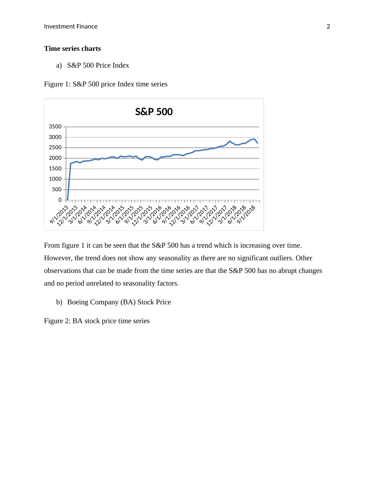
Figure 1: S&P 500 price Index time series
9/1/2013
12/1/2013
3/1/2014
6/1/2014
9/1/2014
12/1/2014
3/1/2015
6/1/2015
9/1/2015
12/1/2015
3/1/2016
6/1/2016
9/1/2016
12/1/2016
3/1/2017
6/1/2017
9/1/2017
12/1/2017
3/1/2018
6/1/2018
9/1/2018
0
500
1000
1500
2000
2500
3000
3500
S&P 500
From figure 1 it can be seen that the S&P 500 has a trend which is increasing over time.
However, the trend does not show any seasonality as there are no significant outliers. Other
observations that can be made from the time series are that the S&P 500 has no abrupt changes
and no period unrelated to seasonality factors.
b) Boeing Company (BA) Stock Price
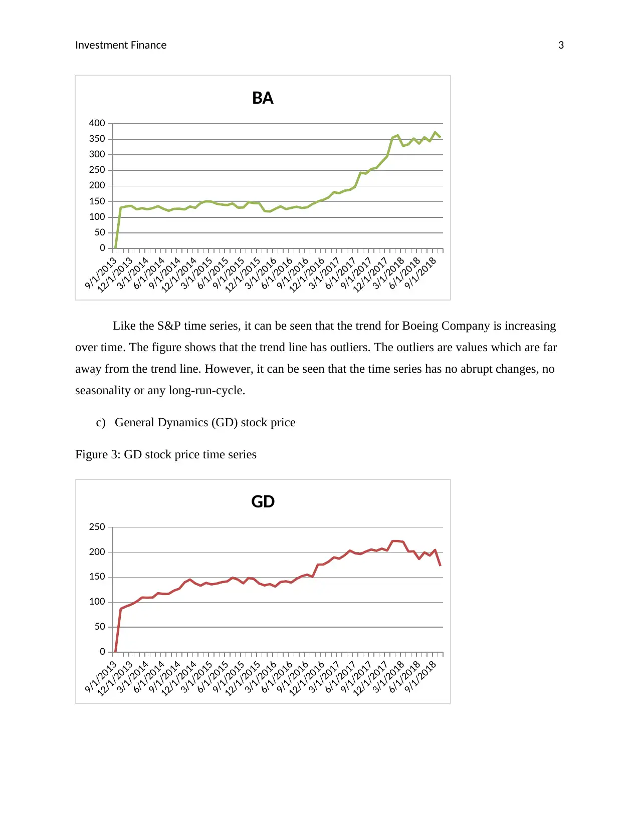
Figure 2: BA stock price time series

Investment Finance 3
9/1/2013
12/1/2013
3/1/2014
6/1/2014
9/1/2014
12/1/2014
3/1/2015
6/1/2015
9/1/2015
12/1/2015
3/1/2016
6/1/2016
9/1/2016
12/1/2016
3/1/2017
6/1/2017
9/1/2017
12/1/2017
3/1/2018
6/1/2018
9/1/2018
0
50
100
150
200
250
300
350
400
BA
Like the S&P time series, it can be seen that the trend for Boeing Company is increasing
over time. The figure shows that the trend line has outliers. The outliers are values which are far
away from the trend line. However, it can be seen that the time series has no abrupt changes, no
seasonality or any long-run-cycle.
c) General Dynamics (GD) stock price
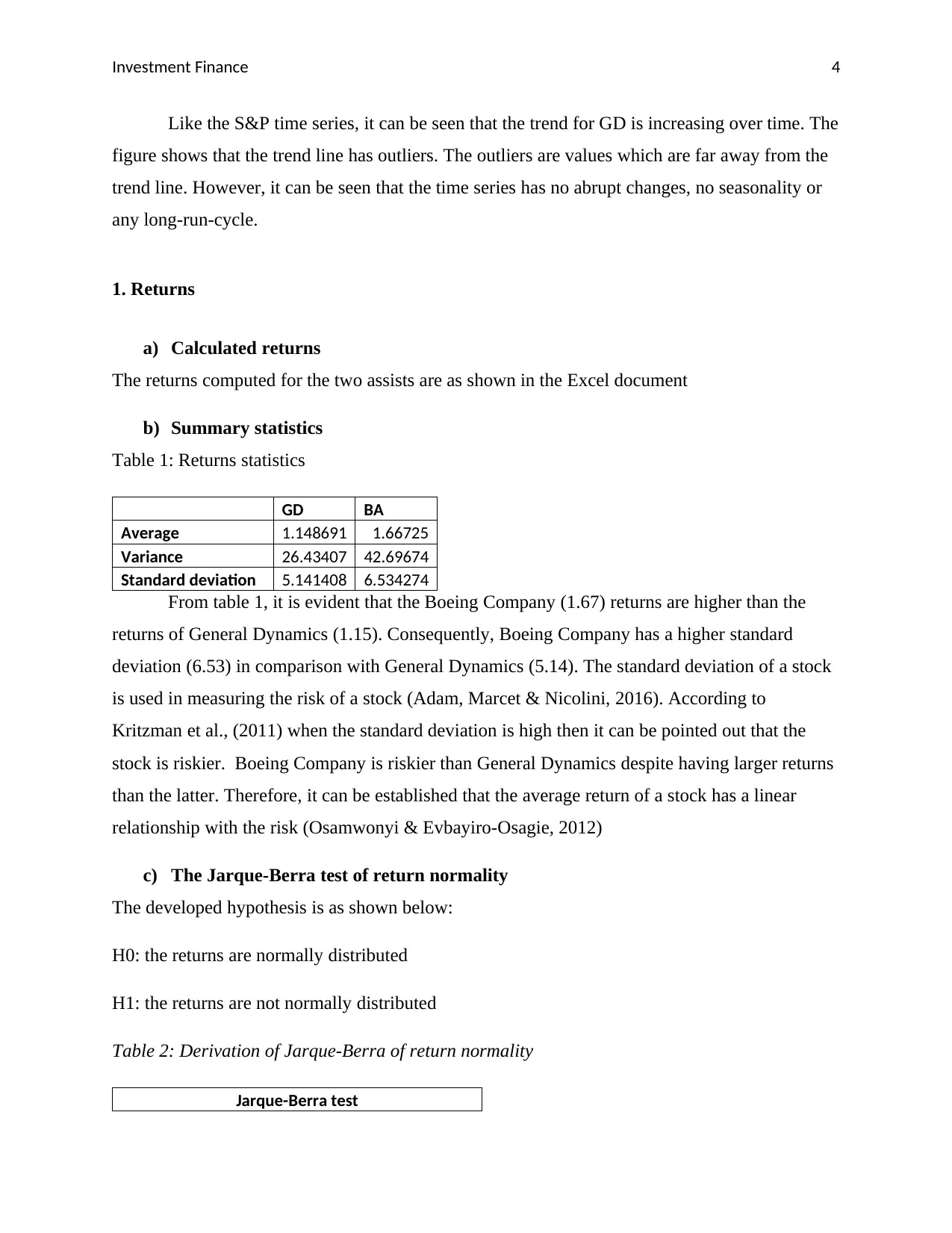
Figure 3: GD stock price time series
9/1/2013
12/1/2013
3/1/2014
6/1/2014
9/1/2014
12/1/2014
3/1/2015
6/1/2015
9/1/2015
12/1/2015
3/1/2016
6/1/2016
9/1/2016
12/1/2016
3/1/2017
6/1/2017
9/1/2017
12/1/2017
3/1/2018
6/1/2018
9/1/2018
0
50
100
150
200
250
GD

Investment Finance 4
Like the S&P time series, it can be seen that the trend for GD is increasing over time. The
figure shows that the trend line has outliers. The outliers are values which are far away from the
trend line. However, it can be seen that the time series has no abrupt changes, no seasonality or
any long-run-cycle.
1. Returns
a) Calculated returns
The returns computed for the two assists are as shown in the Excel document
b) Summary statistics
Table 1: Returns statistics
GD BA
Average 1.148691 1.66725
Variance 26.43407 42.69674
Standard deviation 5.141408 6.534274
From table 1, it is evident that the Boeing Company (1.67) returns are higher than the
returns of General Dynamics (1.15). Consequently, Boeing Company has a higher standard
deviation (6.53) in comparison with General Dynamics (5.14). The standard deviation of a stock
is used in measuring the risk of a stock (Adam, Marcet & Nicolini, 2016). According to
Kritzman et al., (2011) when the standard deviation is high then it can be pointed out that the
stock is riskier. Boeing Company is riskier than General Dynamics despite having larger returns
than the latter. Therefore, it can be established that the average return of a stock has a linear
relationship with the risk (Osamwonyi & Evbayiro-Osagie, 2012)
c) The Jarque-Berra test of return normality
The developed hypothesis is as shown below:
H0: the returns are normally distributed
H1: the returns are not normally distributed
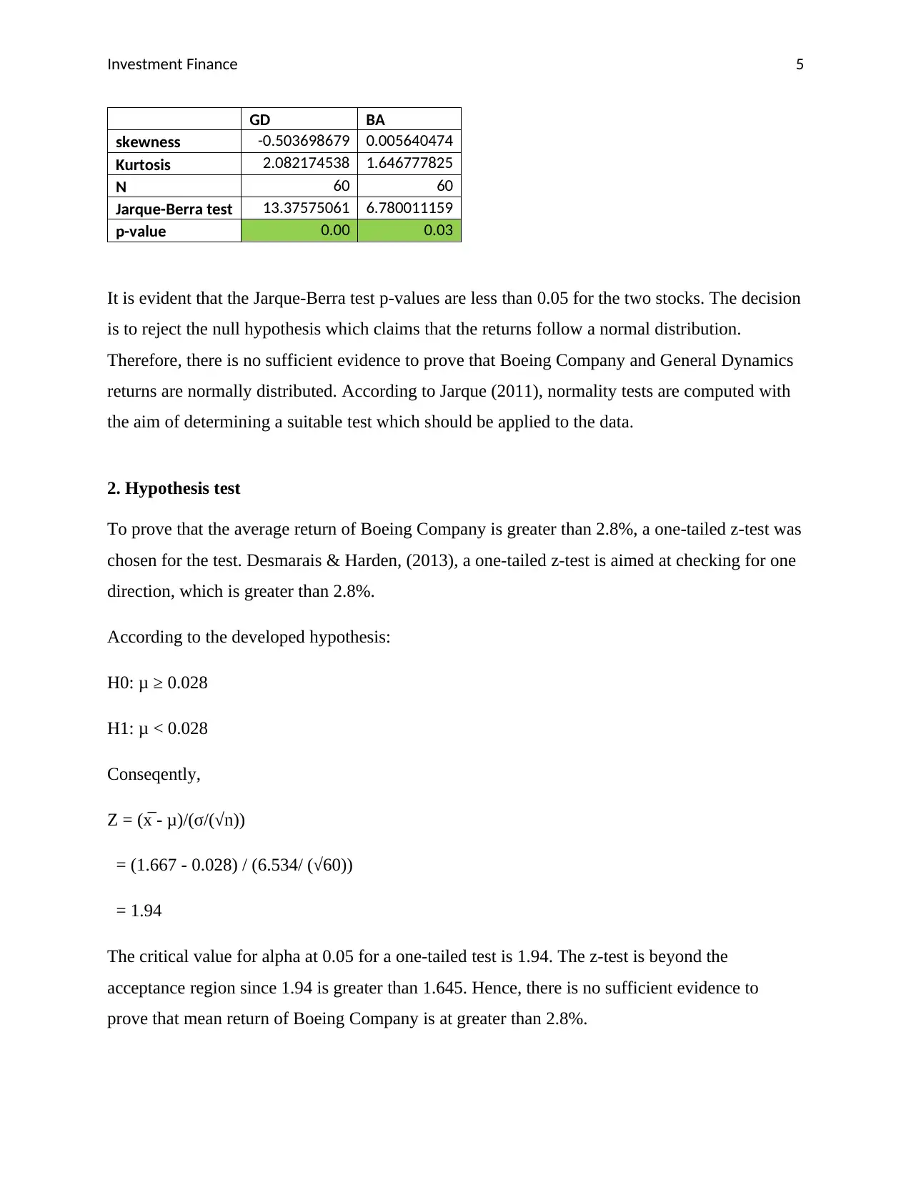
Table 2: Derivation of Jarque-Berra of return normality
Jarque-Berra test

Investment Finance 5
GD BA
skewness -0.503698679 0.005640474
Kurtosis 2.082174538 1.646777825
N 60 60
Jarque-Berra test 13.37575061 6.780011159
p-value 0.00 0.03
It is evident that the Jarque-Berra test p-values are less than 0.05 for the two stocks. The decision
is to reject the null hypothesis which claims that the returns follow a normal distribution.
Therefore, there is no sufficient evidence to prove that Boeing Company and General Dynamics
returns are normally distributed. According to Jarque (2011), normality tests are computed with
the aim of determining a suitable test which should be applied to the data.
2. Hypothesis test
To prove that the average return of Boeing Company is greater than 2.8%, a one-tailed z-test was
chosen for the test. Desmarais & Harden, (2013), a one-tailed z-test is aimed at checking for one
direction, which is greater than 2.8%.
According to the developed hypothesis:
H0: μ ≥ 0.028
H1: μ < 0.028
Conseqently,
Z = (x̅ - μ)/(σ/(√n))
= (1.667 - 0.028) / (6.534/ (√60))
= 1.94
The critical value for alpha at 0.05 for a one-tailed test is 1.94. The z-test is beyond the
acceptance region since 1.94 is greater than 1.645. Hence, there is no sufficient evidence to
prove that mean return of Boeing Company is at greater than 2.8%.

Investment Finance 6
3. Comparison of risk
A chi-square test was adopted to relate the risk related to each of the two stocks. According to
McHugh (2013), the chi-square test is the most suitable since it tests the connection between
categorical variables.
Thus,
H0: σ1 = σ2
H1: σ1 ≠ σ2
Denominator degree of freedom = 60 -1 = 59
Numerator degree of freedom = 60 - 1 = 59
α = 0.05
F = σ2 1
σ2 2 = 26.43 / 42.70 = 0.619
Critical values: F (0.975, 59, 59) = 0.597
F (0.025, 59, 59) =1.674
Rejection region: Reject H0 if F < 0.54 or F > 1.0
From the above results, it is evident that the decision is to accept the null hypothesis since the F
statistic is within the acceptance region. Hence, the risks associated with the stock are similar to
each other.
4. Population average return
An ANOVA analysis was chosen to decide whether the average returns of the population are
equal (Zhang & Liang, 2014).
The developed hypothesis is:

Investment Finance 7
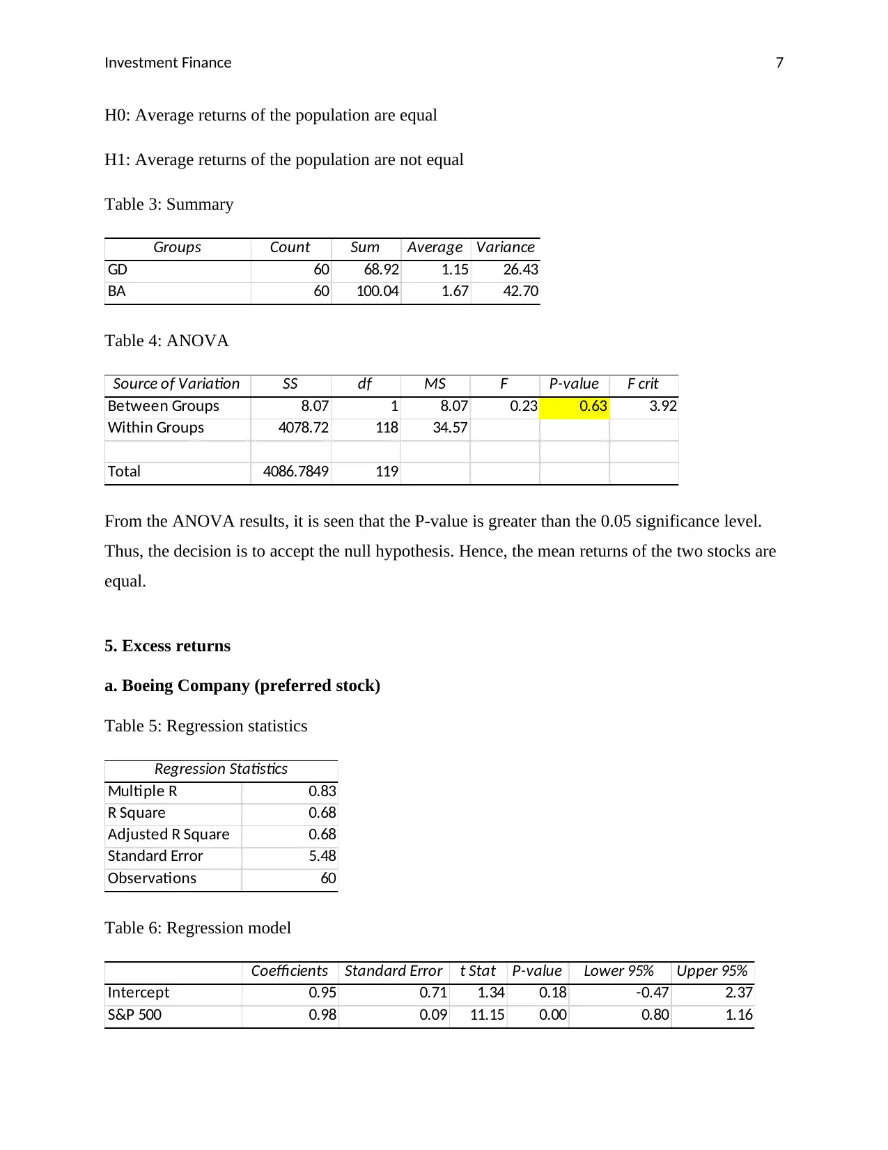
H0: Average returns of the population are equal
H1: Average returns of the population are not equal
Table 3: Summary
Groups Count Sum Average Variance
GD 60 68.92 1.15 26.43
BA 60 100.04 1.67 42.70
Table 4: ANOVA
Source of Variation SS df MS F P-value F crit
Between Groups 8.07 1 8.07 0.23 0.63 3.92
Within Groups 4078.72 118 34.57
Total 4086.7849 119
From the ANOVA results, it is seen that the P-value is greater than the 0.05 significance level.
Thus, the decision is to accept the null hypothesis. Hence, the mean returns of the two stocks are
equal.
5. Excess returns
a. Boeing Company (preferred stock)
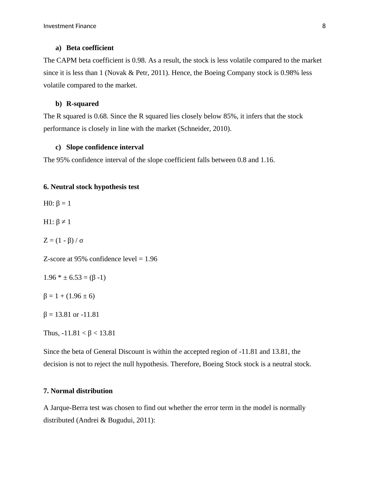
Table 5: Regression statistics
Regression Statistics
Multiple R 0.83
R Square 0.68
Adjusted R Square 0.68
Standard Error 5.48
Observations 60
Table 6: Regression model
Coefficients Standard Error t Stat P-value Lower 95% Upper 95%
Intercept 0.95 0.71 1.34 0.18 -0.47 2.37
S&P 500 0.98 0.09 11.15 0.00 0.80 1.16

Investment Finance 8
a) Beta coefficient
The CAPM beta coefficient is 0.98. As a result, the stock is less volatile compared to the market
since it is less than 1 (Novak & Petr, 2011). Hence, the Boeing Company stock is 0.98% less
volatile compared to the market.
b) R-squared
The R squared is 0.68. Since the R squared lies closely below 85%, it infers that the stock
performance is closely in line with the market (Schneider, 2010).
c) Slope confidence interval
The 95% confidence interval of the slope coefficient falls between 0.8 and 1.16.
6. Neutral stock hypothesis test
H0: β = 1
H1: β ≠ 1
Z = (1 - β) / σ
Z-score at 95% confidence level = 1.96
1.96 * ± 6.53 = (β -1)
β = 1 + (1.96 ± 6)
β = 13.81 or -11.81
Thus, -11.81 < β < 13.81
Since the beta of General Discount is within the accepted region of -11.81 and 13.81, the
decision is not to reject the null hypothesis. Therefore, Boeing Stock stock is a neutral stock.
7. Normal distribution
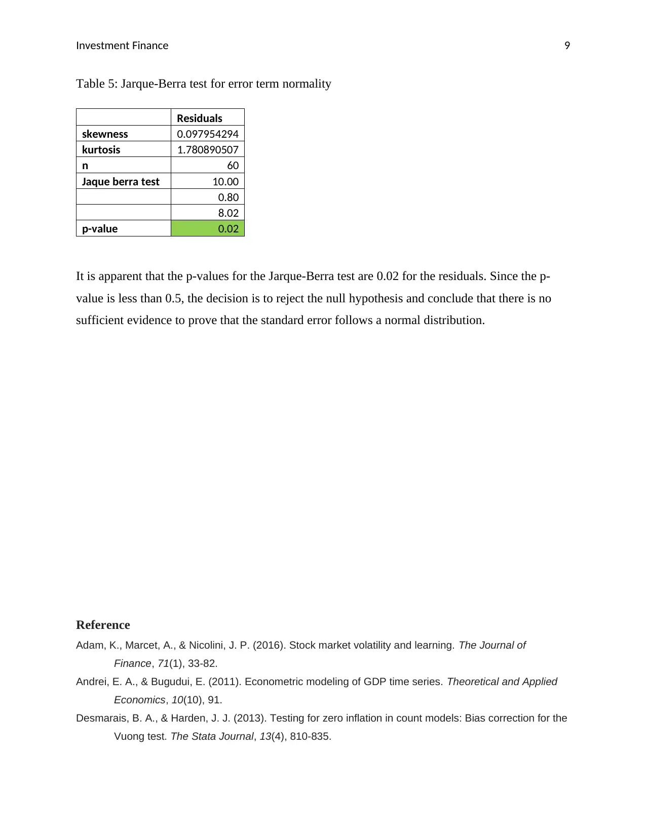
A Jarque-Berra test was chosen to find out whether the error term in the model is normally
distributed (Andrei & Bugudui, 2011):

Investment Finance 9
Table 5: Jarque-Berra test for error term normality
Residuals
skewness 0.097954294
kurtosis 1.780890507
n 60
Jaque berra test 10.00
0.80
8.02
p-value 0.02
It is apparent that the p-values for the Jarque-Berra test are 0.02 for the residuals. Since the p-
value is less than 0.5, the decision is to reject the null hypothesis and conclude that there is no
sufficient evidence to prove that the standard error follows a normal distribution.
Reference
Adam, K., Marcet, A., & Nicolini, J. P. (2016). Stock market volatility and learning. The Journal of
Finance, 71(1), 33-82.
Andrei, E. A., & Bugudui, E. (2011). Econometric modeling of GDP time series. Theoretical and Applied
Economics, 10(10), 91.
Desmarais, B. A., & Harden, J. J. (2013). Testing for zero inflation in count models: Bias correction for the
Vuong test. The Stata Journal, 13(4), 810-835.

Investment Finance 10
Kritzman, M., Li, Y., Page, S., & Rigobon, R. (2011). Principal components as a measure of systemic
risk. The Journal of Portfolio Management, 37(4), 112-126.
Jarque, C. M. (2011). Jarque-bera test. International Encyclopedia of Statistical Science, 701-702.
McHugh, M. L. (2013). The chi-square test of independence. Biochemia medica: Biochemia
medica, 23(2), 143-149.
Novak, J., & Petr, D. (2011). CAPM Beta, Size, Book-to-Market, and Momentum in Realized Stock
Returns. Finance a Uver: Czech Journal of Economics & Finance, 61(1).
Osamwonyi, I. O., & Evbayiro-Osagie, E. I. (2012). The relationship between macroeconomic variables
and stock market index in Nigeria. Journal of Economics, 3(1), 55-63.
Schneider, S. (2010). Investments of Speculative Capital in Staple Foods: Effects and Implications
Exemplified by the Case of Corn. Diplomarbeiten Agentur.
Zhang, J. T., & Liang, X. (2014). One‐way ANOVA for functional data via globalizing the pointwise F‐
test. Scandinavian Journal of Statistics, 41(1), 51-71.