Statistical Analysis of Residential Property Prices: Assignment

This assignment provides a comprehensive statistical analysis of residential property prices. It begins with a hypothesis test comparing average prices in two cities using a two-sample t-test, concluding no significant difference. The second part analyzes the relationship between house prices and intern...Read More

Question 1
The objective is to ascertain if there is any significant difference in the average prices of
residential properties in Coastal City 2 situated in State A and Coastal City 1 situated in State
B.
The relevant hypotheses are as stated below.
H0(Null Hypothesis): μCity 2 = μCity 1
H1(Alternative Hypothesis): μCity 2 ≠ μCity 1
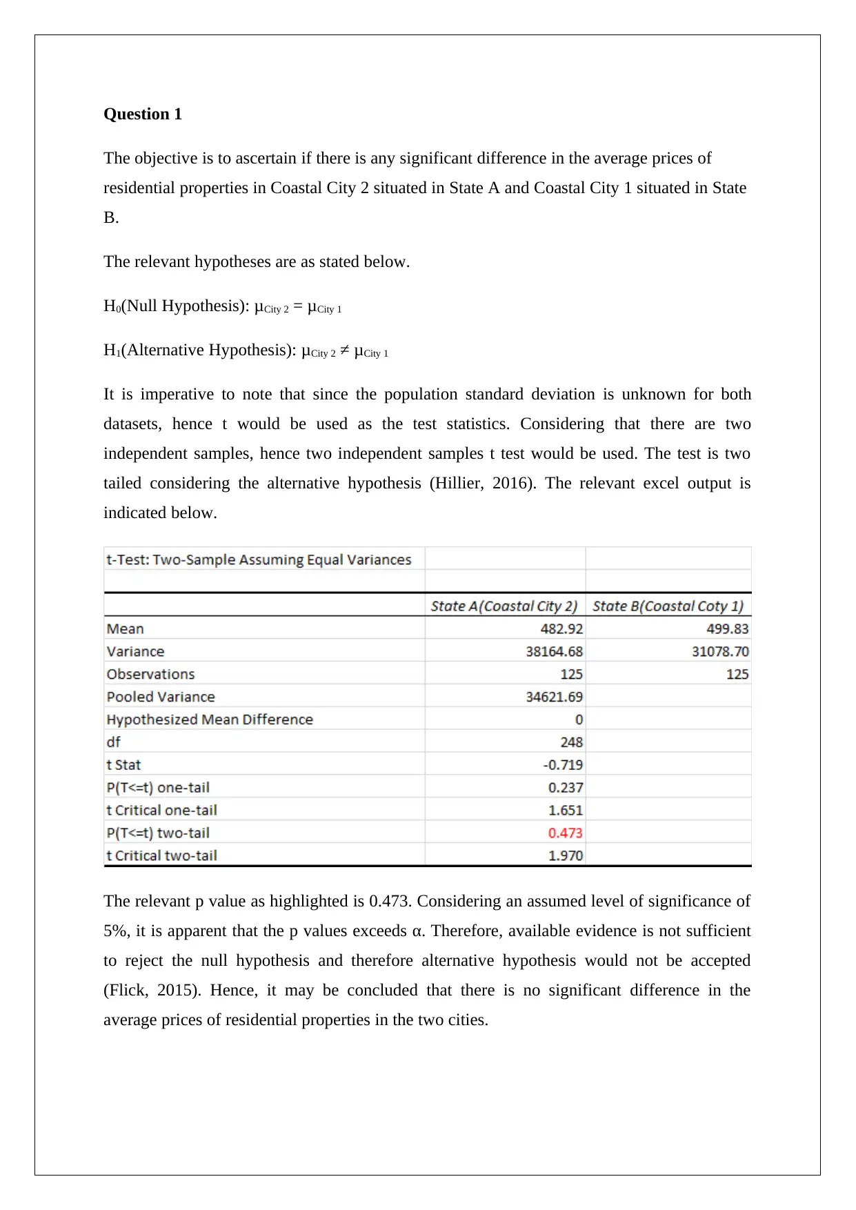
It is imperative to note that since the population standard deviation is unknown for both
datasets, hence t would be used as the test statistics. Considering that there are two
independent samples, hence two independent samples t test would be used. The test is two
tailed considering the alternative hypothesis (Hillier, 2016). The relevant excel output is
indicated below.
The relevant p value as highlighted is 0.473. Considering an assumed level of significance of
5%, it is apparent that the p values exceeds α. Therefore, available evidence is not sufficient
to reject the null hypothesis and therefore alternative hypothesis would not be accepted
(Flick, 2015). Hence, it may be concluded that there is no significant difference in the
average prices of residential properties in the two cities.

Question 2
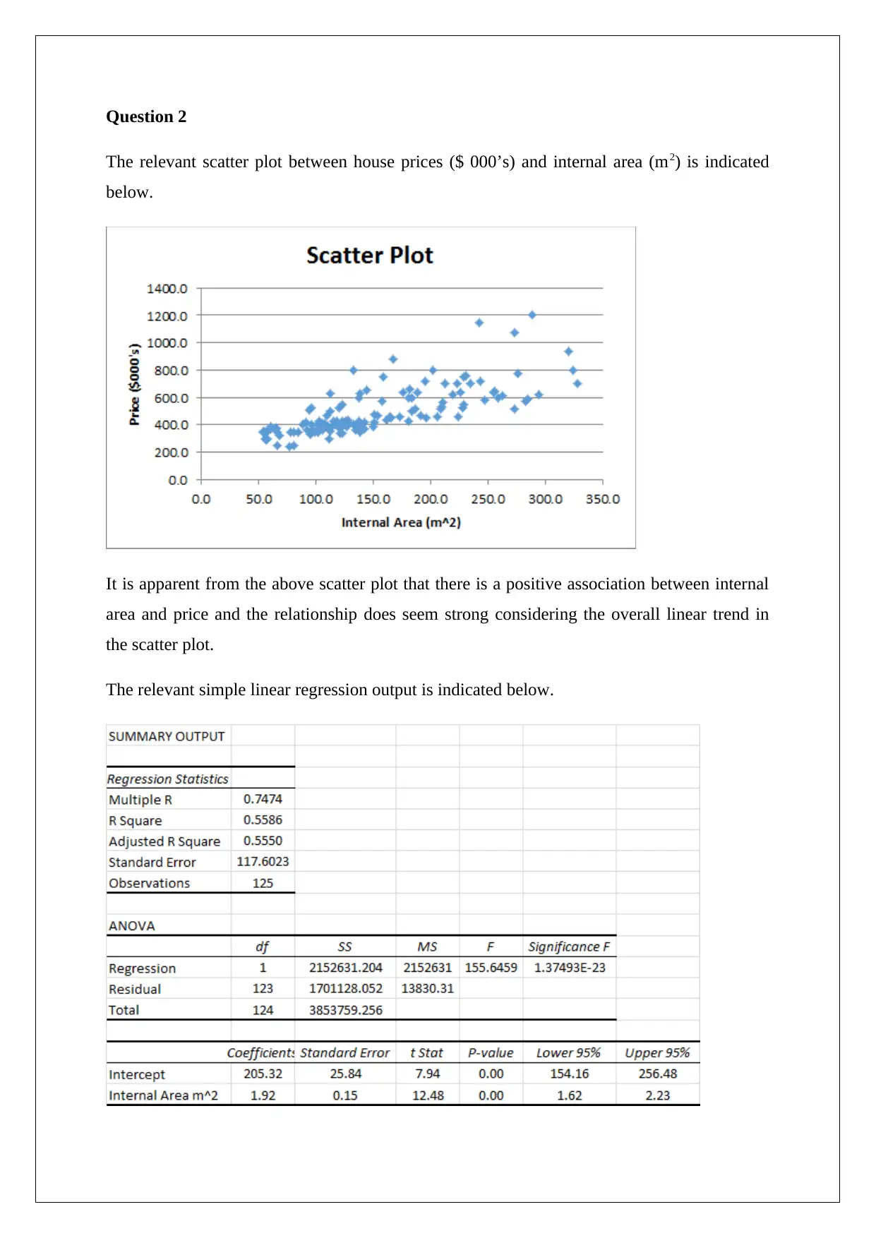
The relevant scatter plot between house prices ($ 000’s) and internal area (m2) is indicated
below.
It is apparent from the above scatter plot that there is a positive association between internal
area and price and the relationship does seem strong considering the overall linear trend in
the scatter plot.
The relevant simple linear regression output is indicated below.

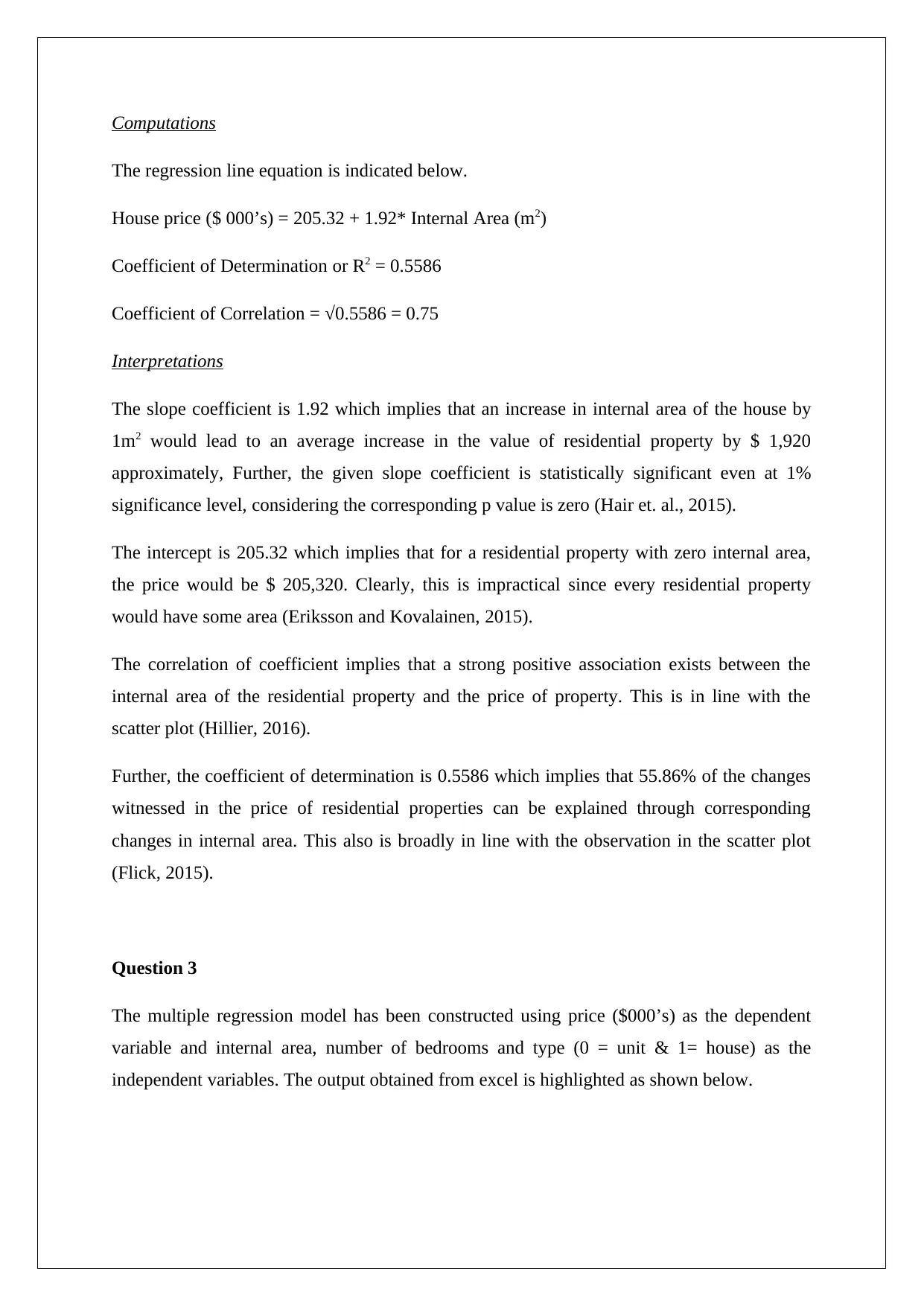
Computations
The regression line equation is indicated below.
House price ($ 000’s) = 205.32 + 1.92* Internal Area (m2)
Coefficient of Determination or R2 = 0.5586
Coefficient of Correlation = √0.5586 = 0.75
Interpretations
The slope coefficient is 1.92 which implies that an increase in internal area of the house by
1m2 would lead to an average increase in the value of residential property by $ 1,920
approximately, Further, the given slope coefficient is statistically significant even at 1%
significance level, considering the corresponding p value is zero (Hair et. al., 2015).
The intercept is 205.32 which implies that for a residential property with zero internal area,
the price would be $ 205,320. Clearly, this is impractical since every residential property
would have some area (Eriksson and Kovalainen, 2015).
The correlation of coefficient implies that a strong positive association exists between the
internal area of the residential property and the price of property. This is in line with the
scatter plot (Hillier, 2016).
Further, the coefficient of determination is 0.5586 which implies that 55.86% of the changes
witnessed in the price of residential properties can be explained through corresponding
changes in internal area. This also is broadly in line with the observation in the scatter plot
(Flick, 2015).
Question 3
The multiple regression model has been constructed using price ($000’s) as the dependent
variable and internal area, number of bedrooms and type (0 = unit & 1= house) as the
independent variables. The output obtained from excel is highlighted as shown below.

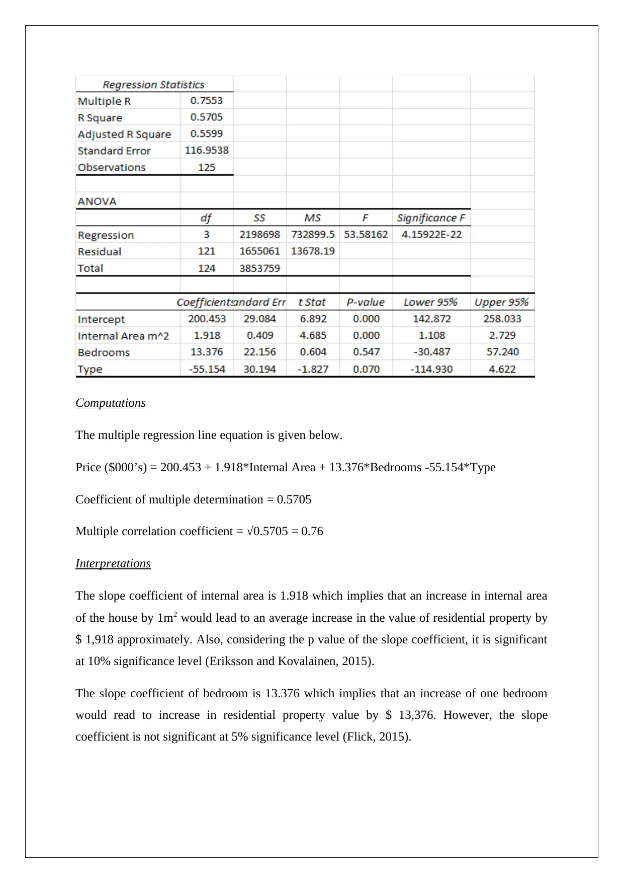
Computations
The multiple regression line equation is given below.
Price ($000’s) = 200.453 + 1.918*Internal Area + 13.376*Bedrooms -55.154*Type
Coefficient of multiple determination = 0.5705
Multiple correlation coefficient = √0.5705 = 0.76
Interpretations
The slope coefficient of internal area is 1.918 which implies that an increase in internal area
of the house by 1m2 would lead to an average increase in the value of residential property by
$ 1,918 approximately. Also, considering the p value of the slope coefficient, it is significant
at 10% significance level (Eriksson and Kovalainen, 2015).
The slope coefficient of bedroom is 13.376 which implies that an increase of one bedroom
would read to increase in residential property value by $ 13,376. However, the slope
coefficient is not significant at 5% significance level (Flick, 2015).

The slope coefficient of type is -55.154 which implies that a house on an average is price
$55,154 lower than the unit with similar other attributes. The p value highlights that slope is
significant at 10% significance level (Hillier, 2016).
The coefficient of determination implies that 57.05% of all variations in price of residential
properties can be jointly explained by internal area, number of bedrooms and type. The
multiple correlation coefficient also suggests that a strong association result is present (Hair
et. al., 2015).
Best Model
Considering that R2 and R tend to be higher for multiple regression model as compared to
simple regression model, hence the multiple regression model represents the best model. The
significance of the slope of the type independent variable also provides evidence in this
regards (Hastie, Tibshirani and Friedman, 2011).

References
Eriksson, P. and Kovalainen, A. (2015) Quantitative methods in business research 3rd ed.
London: Sage Publications.
Flick, U. (2015) Introducing research methodology: A beginner's guide to doing a research
project. 4th ed. New York: Sage Publications.
Hair, J. F., Wolfinbarger, M., Money, A. H., Samouel, P., and Page, M. J. (2015) Essentials
of business research methods. 2nd ed. New York: Routledge.
Hastie, T., Tibshirani, R. and Friedman, J. (2011) The Elements of Statistical Learning. 4th
ed. New York: Springer Publications.
Hillier, F. (2016) Introduction to Operations Research. 6th ed. New York: McGraw Hill
Publications.