ENG3104 Assignment 3: Numerical Methods for Engineering Simulation

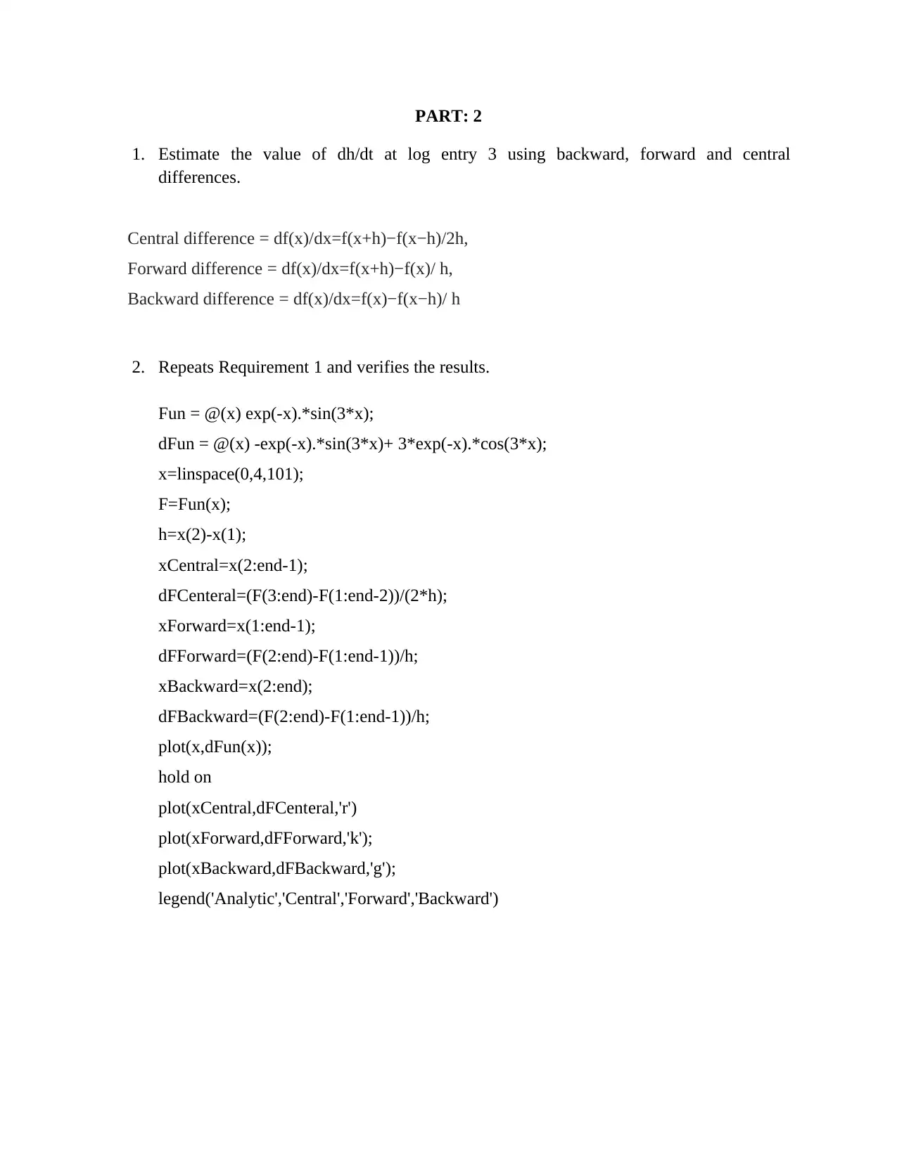
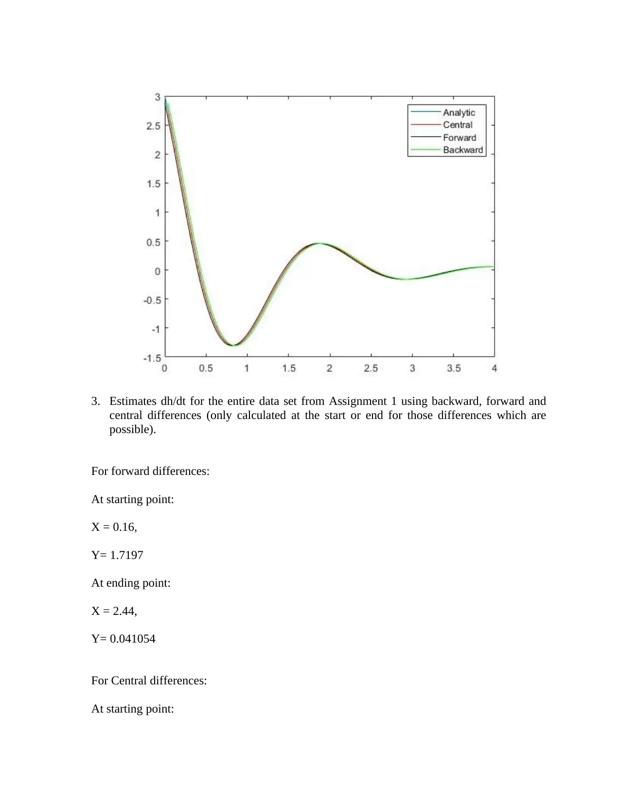
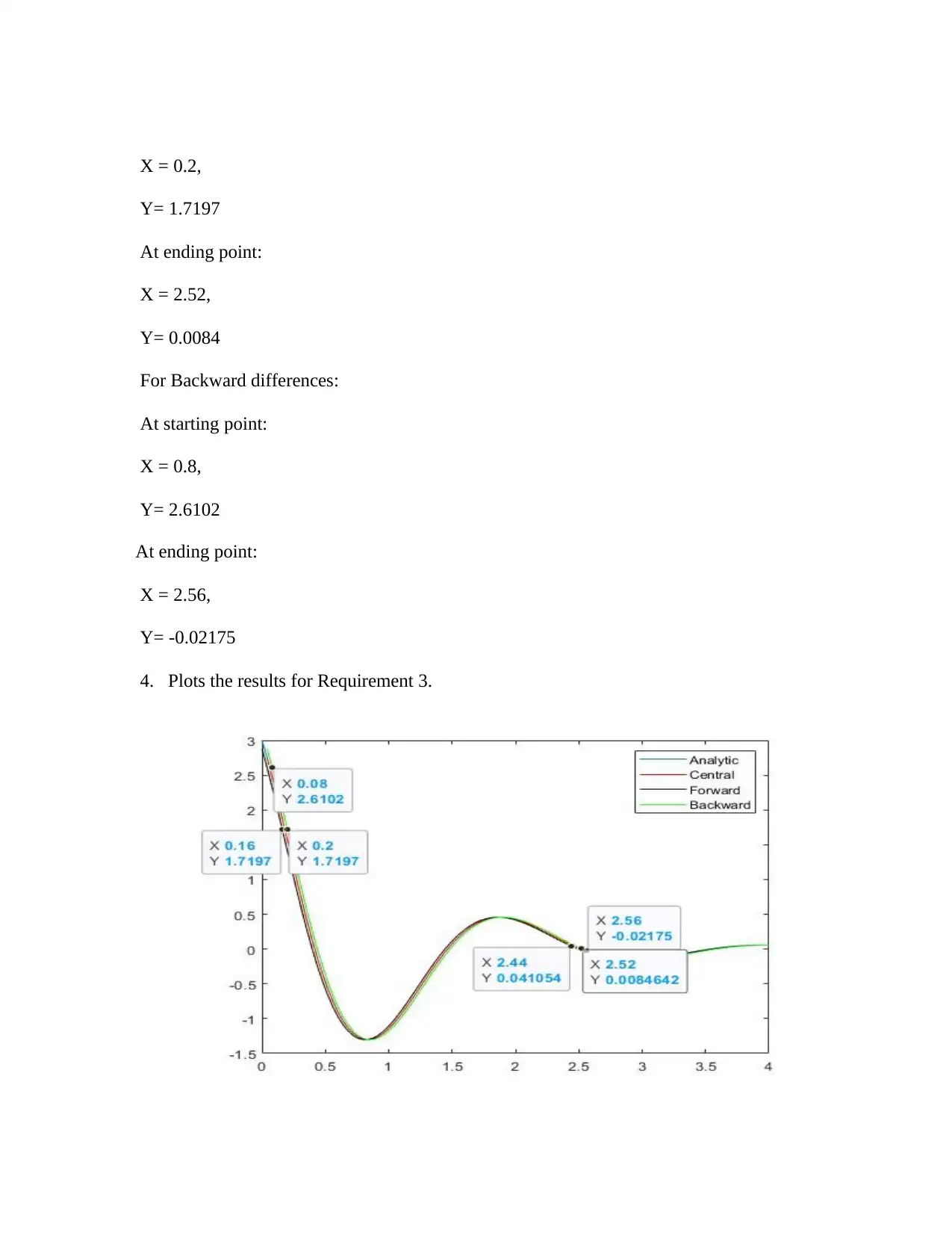
This assignment for ENG3104, Engineering Simulations and Computations, delves into numerical methods and their application in engineering contexts. The assignment requires students to estimate the value of dh/dt using backward, forward, and central differences, analyze the results, and determine the best method. It further involves estimating accelerations, finding the actual total impulse analytically using the trapezoidal method, and validating the results. Students are tasked with plotting results, conducting mesh-independence studies, and comparing planned versus actual fuel consumption in a simulation. The provided solution demonstrates the application of these methods using MATLAB, including code snippets, plots, and detailed explanations of each step. The assignment covers a wide range of numerical techniques essential for engineering analysis and simulation.

PART: 2
1. Estimate the value of dh/dt at log entry 3 using backward, forward and central
differences.
Central difference = df(x)/dx=f(x+h)−f(x−h)/2h,
Forward difference = df(x)/dx=f(x+h)−f(x)/ h,
Backward difference = df(x)/dx=f(x)−f(x−h)/ h
2. Repeats Requirement 1 and verifies the results.
Fun = @(x) exp(-x).*sin(3*x);
dFun = @(x) -exp(-x).*sin(3*x)+ 3*exp(-x).*cos(3*x);
x=linspace(0,4,101);
F=Fun(x);
h=x(2)-x(1);
xCentral=x(2:end-1);
dFCenteral=(F(3:end)-F(1:end-2))/(2*h);
xForward=x(1:end-1);
dFForward=(F(2:end)-F(1:end-1))/h;
xBackward=x(2:end);
dFBackward=(F(2:end)-F(1:end-1))/h;
plot(x,dFun(x));
hold on
plot(xCentral,dFCenteral,'r')
plot(xForward,dFForward,'k');
plot(xBackward,dFBackward,'g');
legend('Analytic','Central','Forward','Backward')

3. Estimates dh/dt for the entire data set from Assignment 1 using backward, forward and
central differences (only calculated at the start or end for those differences which are
possible).
For forward differences:
At starting point:
X = 0.16,
Y= 1.7197
At ending point:
X = 2.44,
Y= 0.041054
For Central differences:
At starting point:

X = 0.2,
Y= 1.7197
At ending point:
X = 2.52,
Y= 0.0084
For Backward differences:
At starting point:
X = 0.8,
Y= 2.6102
At ending point:
X = 2.56,
Y= -0.02175
4. Plots the results for Requirement 3.

5. Discuss which is the best result out of the backward, forward and central differences and
Why.
Central difference is more preferable than the backward in forward differences. Some of
the main reason of it is mentioning below:
 The central difference scheme is in the second order of h for smooth f, however
the other two is being mentioned in first order of h. The real space error for the
central difference scheme is O(h2) at the time of smooth f whereas for the forward
and the backward scheme it would be O(h). Hence the central difference will have
a better error rather than other two, at the fixed sufficient h.
 Central differences use the points at same numbers rather than other two, by
which there will be no loss in efficiency.
6. Determines the first instant the magnitude of the rate of descent for the central difference
became lower than the value in Eq. (1).
dh /dt = 10 + 4×6.7131 ft/s
At, X= 0.12,
Y= 2.3253

7. Estimates the accelerations in the vertical direction by:
(a) Taking the central difference of the central difference from Requirement 3;
Central Difference:
X = 2
Y= 0.43628
(b) Directly calculating the second derivative.
close all; clear all;
f=@(x) sin(x); x0=0.5;
ed2f=@(x) -sin(x);
dx=[0.5:-0.1:0.1,0.05,0.01,0.005,0.001]; N=length(dx);
d2f=zeros(1,N); Err = zeros(1,N);
for i=1:N
fL=f(x0-dx(i)); f0=f(x0); fR=f(x0+dx(i));

d2f(i)=(fL-2*f0+fR)/dx(i)^2;
Err(i)=100*abs((d2f(i)-ed2f(x0))/ed2f(x0));
end
semilogx(dx,d2f,'b--o',dx,ed2f(x0)*ones(1,N),'m');
legend('Approximate','Exact');
xlabel('\Delta x'); ylabel('d^2f(0.5)/dx^2')
disp('Press any key')
pause
loglog(dx,Err,'bo'); hold on
xlabel('\Delta x'); ylabel('Percentage error')
coef=polyfit(log10(dx),log10(Err),1);
loglog(dx([1,end]),10^coef(2)*dx([1,end]).^coef(1),'m');
8. Has appropriate comments throughout.

>> Fun = @(x) exp(-x).*sin(3*x); % Provide the function value
dFun = @(x) -exp(-x).*sin(3*x)+ 3*exp(-x).*cos(3*x); % Define Function
x=linspace(0,4,101); % Define Variable X
F=Fun(x); % Define Function as f(x)
h=x(2)-x(1); % Define interval h
xCentral=x(2:end-1); % Define the central value for x
dFCenteral=(F(3:end)-F(1:end-2))/(2*h); % Value determination for central difference
xForward=x(1:end-1); % Define the Forward value for x
dFForward=(F(2:end)-F(1:end-1))/h; % Value determination for Forward difference
xBackward=x(2:end); % Define the Backward value for x
dFBackward=(F(2:end)-F(1:end-1))/h; %Value determination for Backward difference
plot(x,dFun(x)); % Plot function of x
hold on % Hold command
plot(xCentral,dFCenteral,'r') %Plot central difference
plot(xForward,dFForward,'k'); % Plot Forward difference
plot(xBackward,dFBackward,'g'); % Plot Backward difference
legend('Analytic','Central','Forward','Backward') %Define lines for parameters
PART: 3

1. Find the actual total impulse analytically.
>> orig_data=read(rfdata.data,'passive.s2p')
orig_data =
rfdata.data with properties:
Freq: [202×1 double]
S_Parameters: [2×2×202 double]
GroupDelay: [202×1 double]
NF: [202×1 double]
OIP3: [202×1 double]
Z0: 50.0000 + 0.0000i
ZS: 50.0000 + 0.0000i
ZL: 50.0000 + 0.0000i
IntpType: 'Linear'
Name: 'Data object'
2. Repeat Requirement 1 using the trapezoidal method with four intervals along the total
duration (the intervals can have different durations). Validate the result with
Requirement 1.
>> close all; clear all;
a=0; b=pi;
esol=2; % Exact answer
n1=input('The minimum number of subintervals/elements: ');
n2=input('The maximum number of subintervals/elements: ');
x0=linspace(a,b,101);
y0=sin(x0);
disp('No of subintervals, Exact solution, Computed solution, Percentage error: ')
for n=n1:n2
x=linspace(a,b,n+1);

y=sin(x);
plot(x0,y0,'b',x,y,'m--o')
sol=trapz(x,y);
fprintf('%3d %6.4f %6.4f %5.2f\n',n, esol, sol, abs((esol-sol)*100/esol))
pause
end
The minimum number of subintervals/elements: 4
The maximum number of subintervals/elements: 4
No of subintervals, Exact solution, Computed solution, Percentage error:
4 2.0000 1.8961 5.19
Validation of the result with Requirement 1:
Here the simulation shows the plot of impulse response but in requirement 1 it shows the value
of impedances such as ZS, Z0, ZL.
3. Plots the actual and planned thrusts.

nx = 6;
ny = 6;
nu = 4;
nlobj = nlmpc(nx,ny,nu);
nlobj.Model.StateFcn = "FlyingRobotStateFcn";
nlobj.Jacobian.StateFcn = @FlyingRobotStateJacobianFcn;
In standard cost function, zero weights are applied by default to one or more OVs
because there are fewer MVs than OVs.
>> Ts = 0.4;
p = 30;
nlobj.Ts = Ts;
nlobj.PredictionHorizon = p;
>> nlobj.ControlHorizon = p;
>> nlobj.Optimization.CustomCostFcn = @(X,U,e,data) Ts*sum(sum(U(1:p,:)));
nlobj.Optimization.ReplaceStandardCost = true;
>> nlobj.Optimization.CustomEqConFcn = @(X,U,data) X(end,:)';
>> for ct = 1:nu
nlobj.MV(ct).Min = 0;
nlobj.MV(ct).Max = 1;
end
>> x0 = [-10;-10;pi/2;0;0;0]; % robot parks at [-10, -10], facing north
u0 = zeros(nu,1); % thrust is zero
>> validateFcns(nlobj,x0,u0);
Model.StateFcn is OK.
Jacobian.StateFcn is OK.
No output function specified. Assuming "y = x" in the prediction model.
Optimization.CustomCostFcn is OK.
Optimization.CustomEqConFcn is OK.
Analysis of user-provided model, cost, and constraint functions complete.
>> [~,~,info] = nlmpcmove(nlobj,x0,u0);

Slack variable unused or zero-weighted in your custom cost function. All constraints
will be hard.
FlyingRobotPlotPlanning(info);
Optimal fuel consumption = 7.797825