[SOLVED] Regression Analysis of Stock Prices

This document provides the results of a regression analysis on stock prices, including coefficients, standard errors, t-statistics, and probabilities. The analysis includes variables RP_MKT, RP_C, RP_IBM, and RP_MEX, with corresponding coefficients, standard errors, t-statistics, and probabilities. It also includes various statistical metrics such as R-squared values, mean dependent variables, adjusted R-squared values, S.D. dependent variables, S.E. of regression, Akaike information criteria, sum squared residuals, Schwarz criteria, log likelihood, Hannan-Quinn criteria, F-statistics, Durbin-Watson statistics, and probabilities.

Estimation and Testing of Capital Asset Pricing Model

TABLE OF CONTENTS
1. Regression analysis..................................................................................................................3
2. Interpreting the estimate of βj from your regression result above...........................................3
3. Testing null hypothesis that αj = 0 for Microsoft stock in against to an appropriate
alternative hypotheses..................................................................................................................3
4. Performing a hypothesis test that βj = 0 against the alternative that βj ≠ 0 using the
Microsoft data..............................................................................................................................3
5. Evaluate whether Microsoft stock (a Tech stock) is an aggressive stock or not by applying
suitable test..................................................................................................................................4
6. Stating R2 for the regression and interpreting the same...........................................................5
7. Stating predicted return in relation to Microsoft for January 2009 if the risk free rate does
not change from December 2008 but the market return increases by 1%...................................5
8. Repeat Question 1 for GE, GM, IBM, Disney, and Mobil-Exxon..........................................5
APPENDIX......................................................................................................................................8
1...................................................................................................................................................8
2...................................................................................................................................................8
3...................................................................................................................................................8

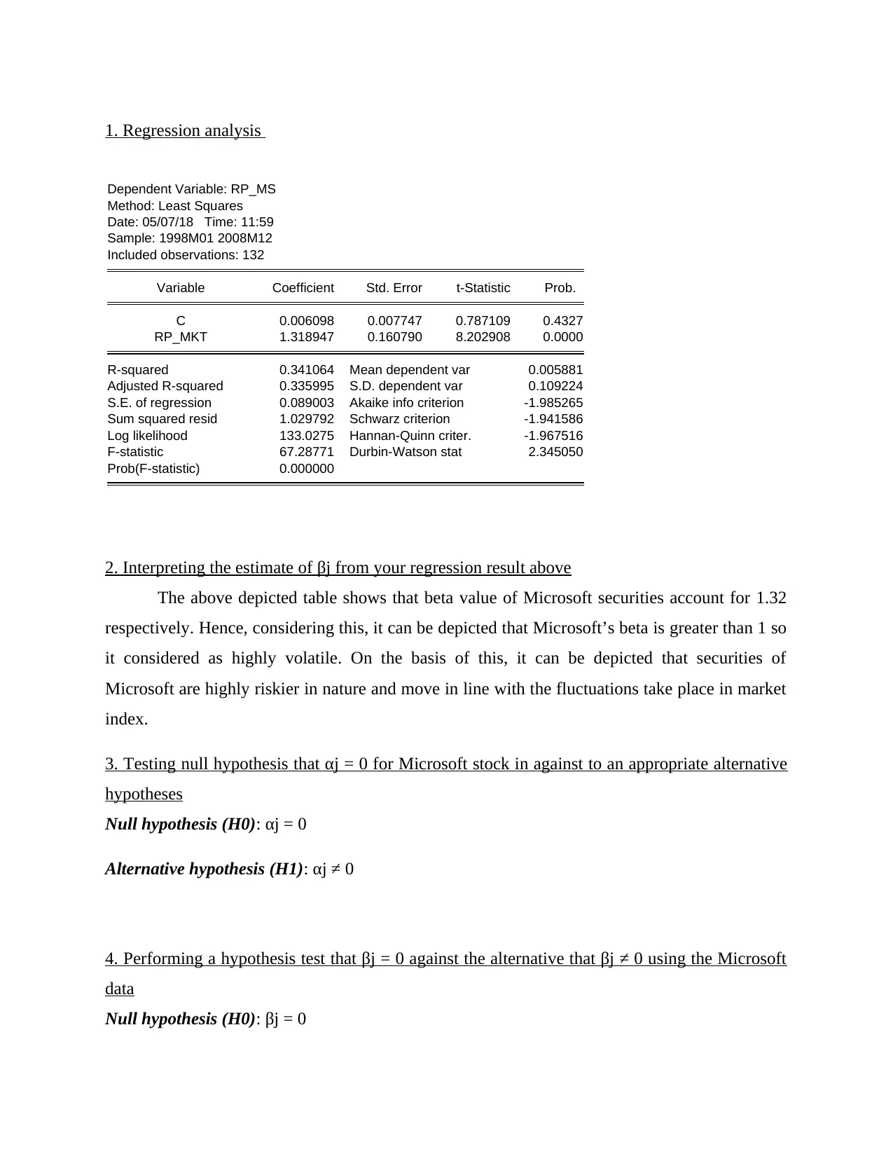
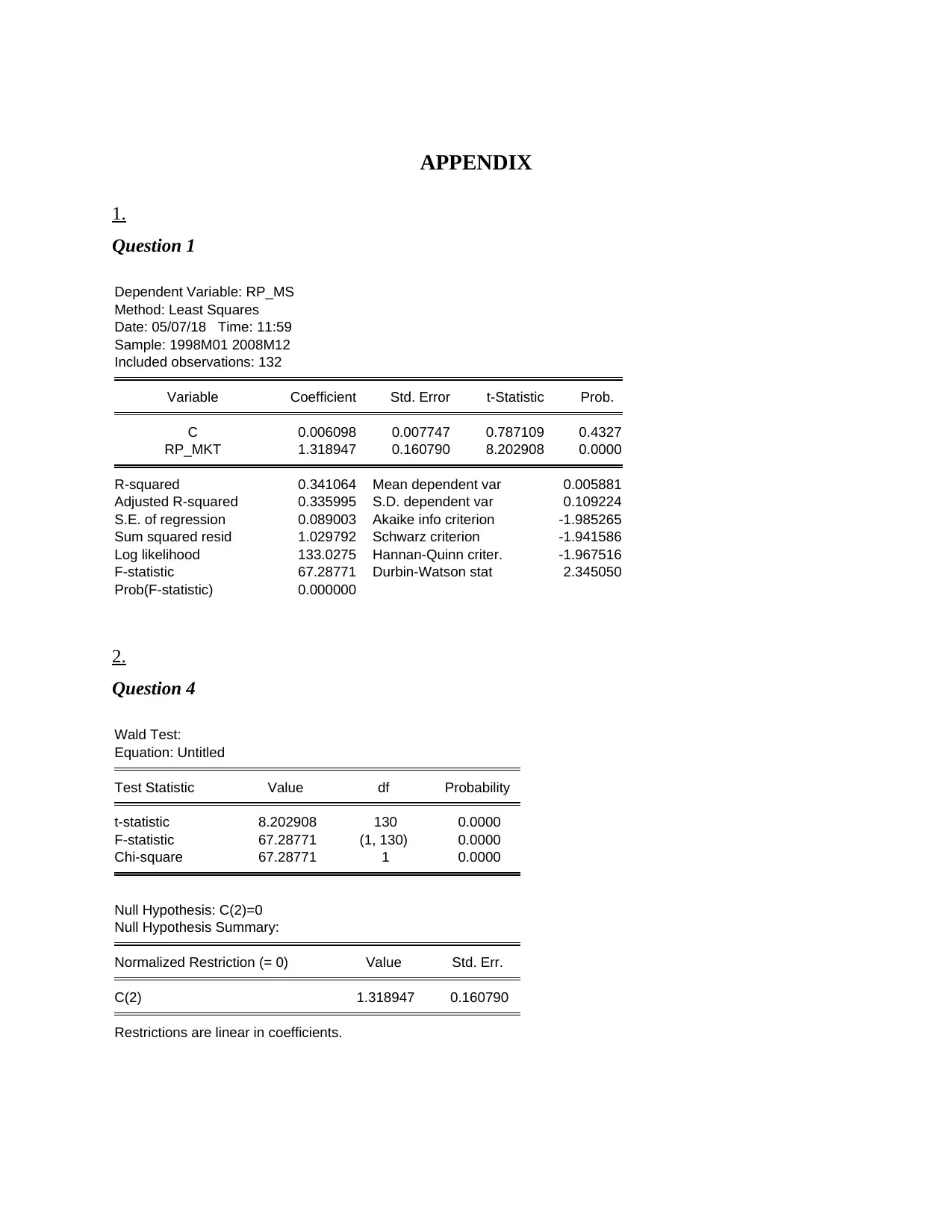
1. Regression analysis
Dependent Variable: RP_MS
Method: Least Squares
Date: 05/07/18 Time: 11:59
Sample: 1998M01 2008M12
Included observations: 132
Variable Coefficient Std. Error t-Statistic Prob.
C 0.006098 0.007747 0.787109 0.4327
RP_MKT 1.318947 0.160790 8.202908 0.0000
R-squared 0.341064 Mean dependent var 0.005881
Adjusted R-squared 0.335995 S.D. dependent var 0.109224
S.E. of regression 0.089003 Akaike info criterion -1.985265
Sum squared resid 1.029792 Schwarz criterion -1.941586
Log likelihood 133.0275 Hannan-Quinn criter. -1.967516
F-statistic 67.28771 Durbin-Watson stat 2.345050
Prob(F-statistic) 0.000000
2. Interpreting the estimate of βj from your regression result above
The above depicted table shows that beta value of Microsoft securities account for 1.32
respectively. Hence, considering this, it can be depicted that Microsoft’s beta is greater than 1 so
it considered as highly volatile. On the basis of this, it can be depicted that securities of
Microsoft are highly riskier in nature and move in line with the fluctuations take place in market
index.
3. Testing null hypothesis that αj = 0 for Microsoft stock in against to an appropriate alternative
hypotheses
Null hypothesis (H0): αj = 0
Alternative hypothesis (H1): αj ≠ 0
4. Performing a hypothesis test that βj = 0 against the alternative that βj ≠ 0 using the Microsoft
data
Null hypothesis (H0): βj = 0

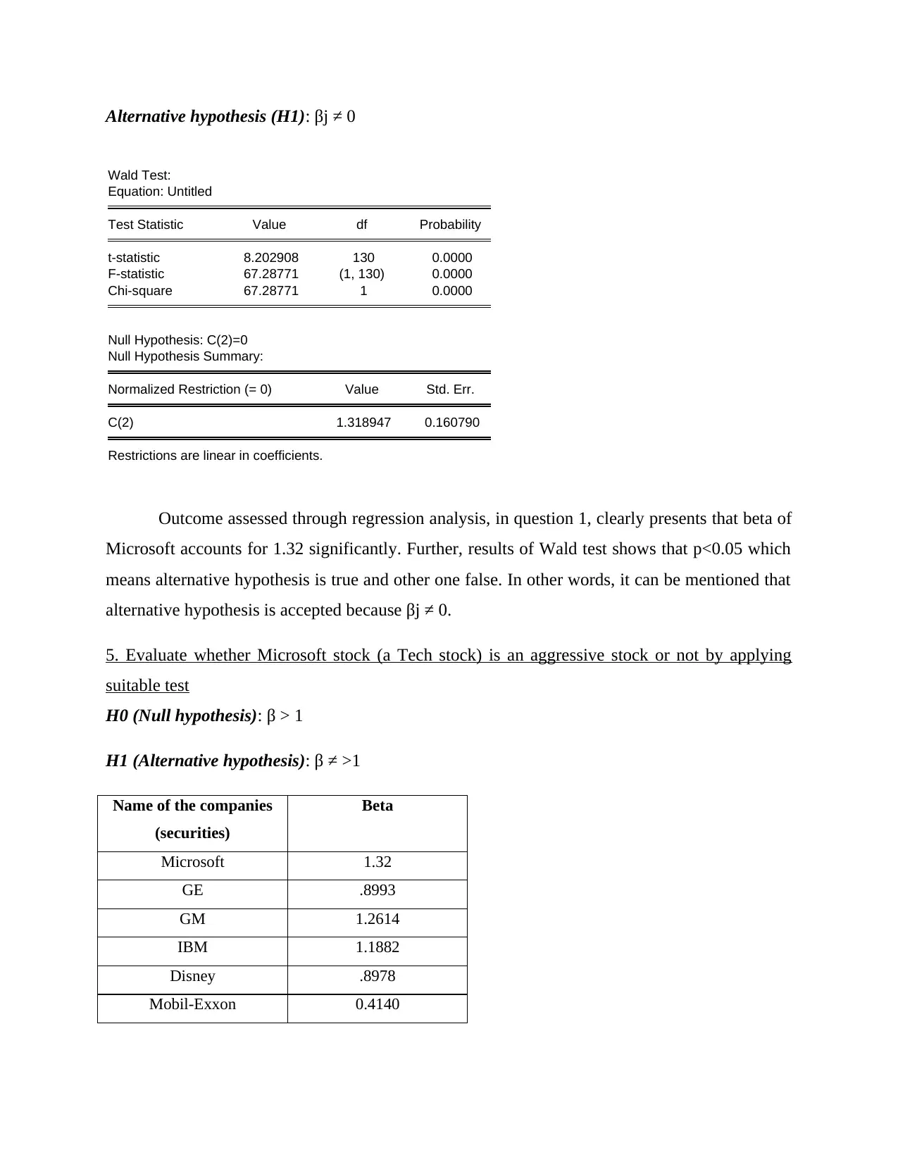
Alternative hypothesis (H1): βj ≠ 0
Wald Test:
Equation: Untitled
Test Statistic Value df Probability
t-statistic 8.202908 130 0.0000
F-statistic 67.28771 (1, 130) 0.0000
Chi-square 67.28771 1 0.0000
Null Hypothesis: C(2)=0
Null Hypothesis Summary:
Normalized Restriction (= 0) Value Std. Err.
C(2) 1.318947 0.160790
Restrictions are linear in coefficients.
Outcome assessed through regression analysis, in question 1, clearly presents that beta of
Microsoft accounts for 1.32 significantly. Further, results of Wald test shows that p<0.05 which
means alternative hypothesis is true and other one false. In other words, it can be mentioned that
alternative hypothesis is accepted because βj ≠ 0.
5. Evaluate whether Microsoft stock (a Tech stock) is an aggressive stock or not by applying
suitable test
H0 (Null hypothesis): β > 1
H1 (Alternative hypothesis): β ≠ >1
Name of the companies
(securities)
Beta
Microsoft 1.32
GE .8993
GM 1.2614
IBM 1.1882
Disney .8978
Mobil-Exxon 0.4140

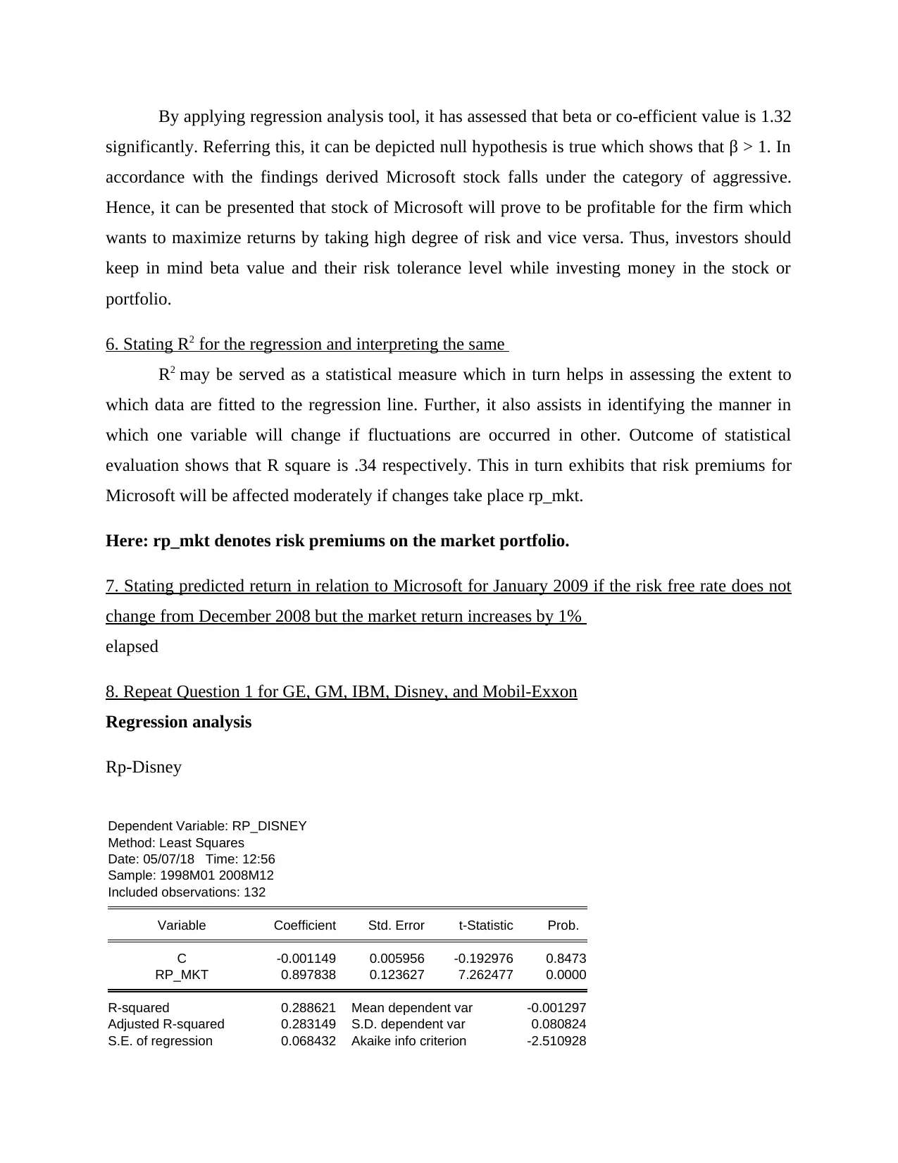
By applying regression analysis tool, it has assessed that beta or co-efficient value is 1.32
significantly. Referring this, it can be depicted null hypothesis is true which shows that β > 1. In
accordance with the findings derived Microsoft stock falls under the category of aggressive.
Hence, it can be presented that stock of Microsoft will prove to be profitable for the firm which
wants to maximize returns by taking high degree of risk and vice versa. Thus, investors should
keep in mind beta value and their risk tolerance level while investing money in the stock or
portfolio.
6. Stating R2 for the regression and interpreting the same
R2 may be served as a statistical measure which in turn helps in assessing the extent to
which data are fitted to the regression line. Further, it also assists in identifying the manner in
which one variable will change if fluctuations are occurred in other. Outcome of statistical
evaluation shows that R square is .34 respectively. This in turn exhibits that risk premiums for
Microsoft will be affected moderately if changes take place rp_mkt.
Here: rp_mkt denotes risk premiums on the market portfolio.
7. Stating predicted return in relation to Microsoft for January 2009 if the risk free rate does not
change from December 2008 but the market return increases by 1%
elapsed
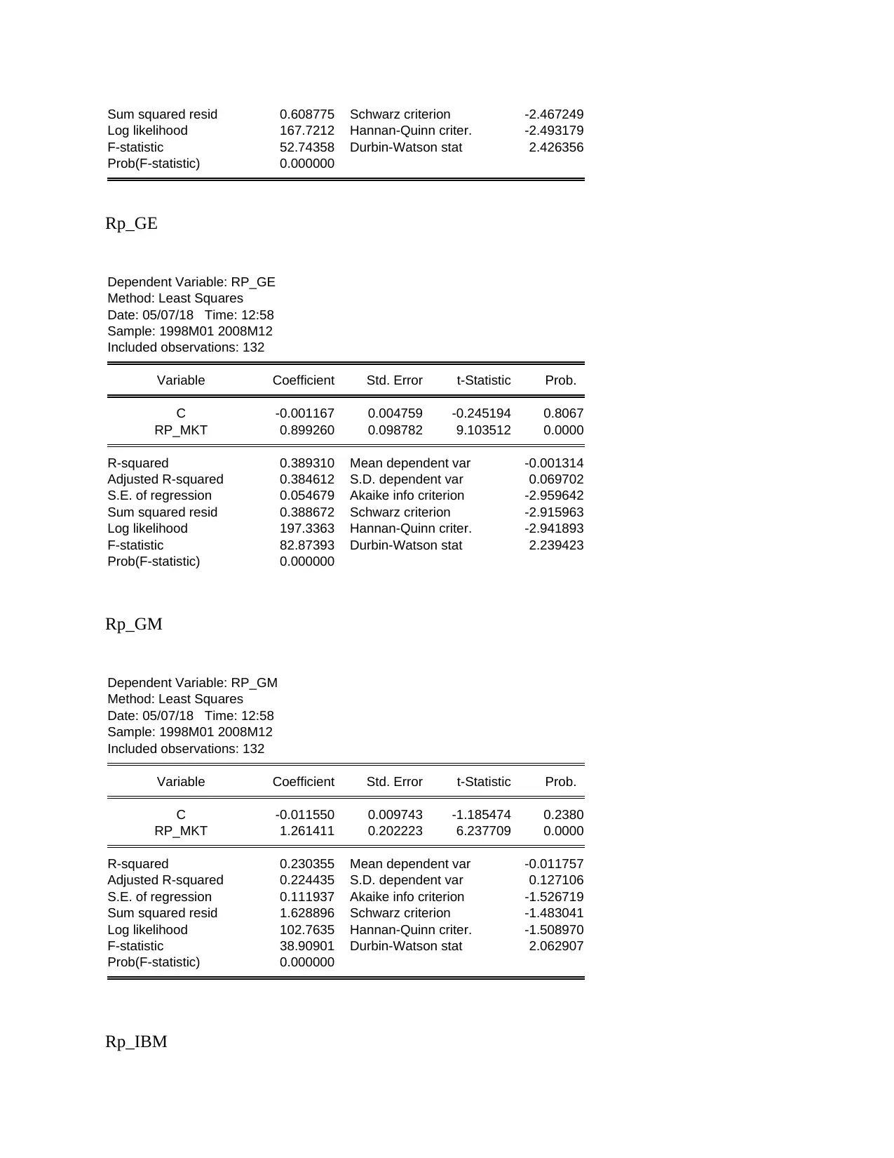
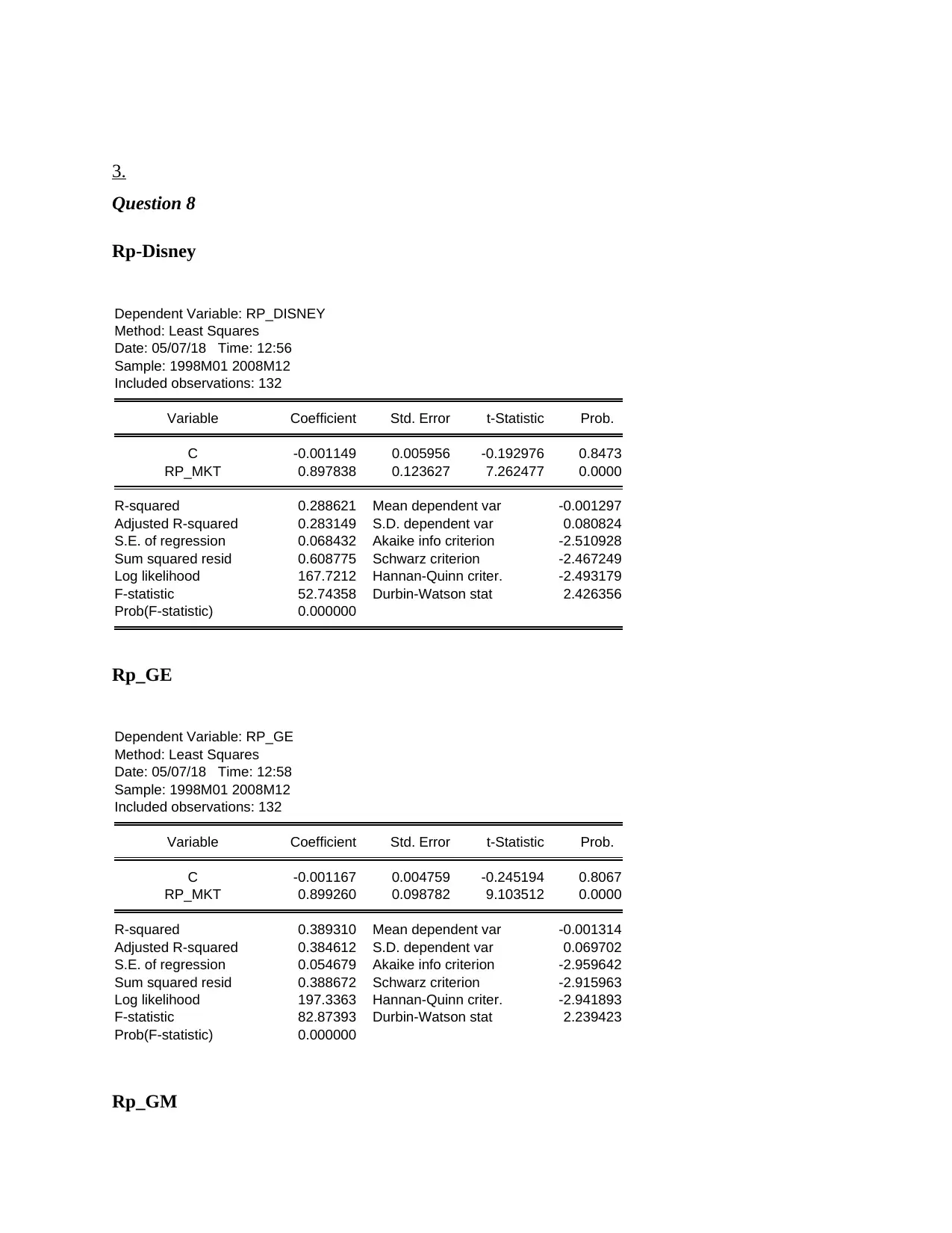
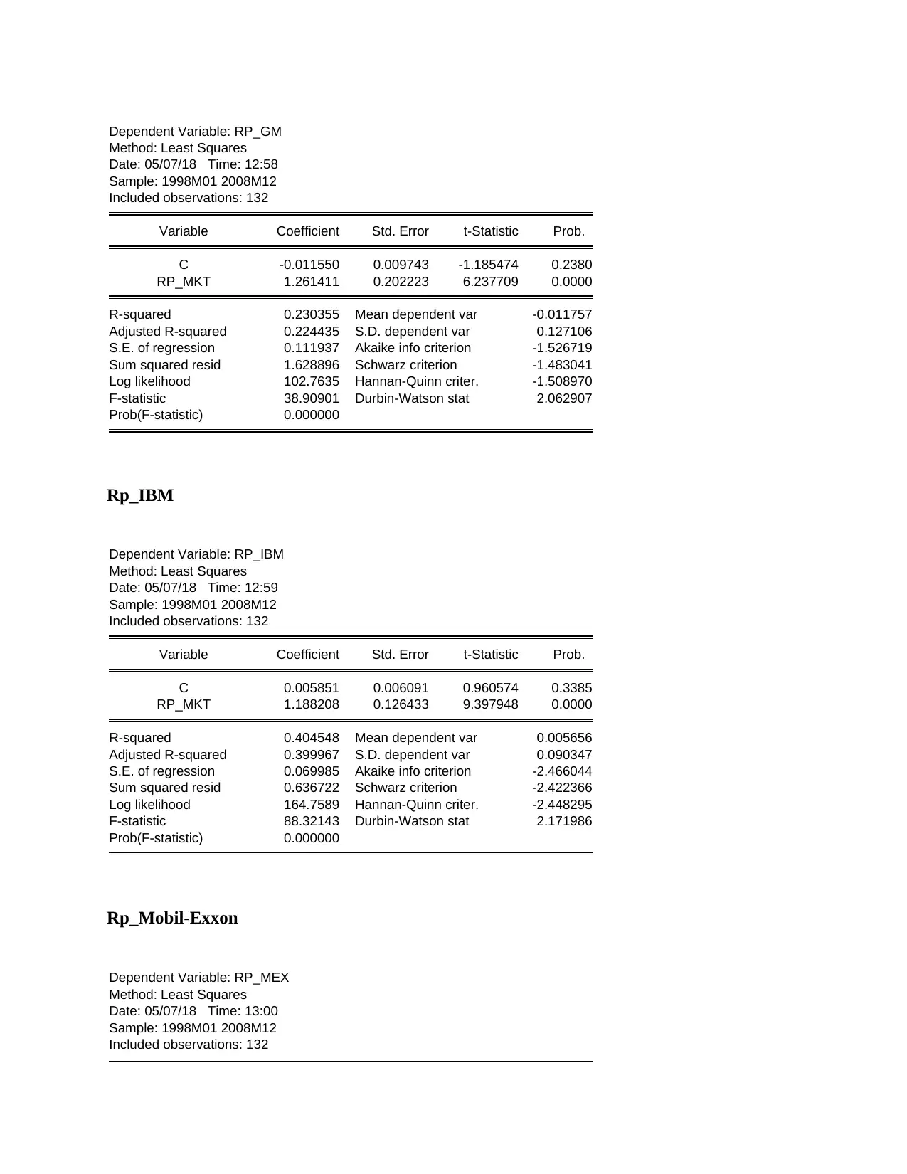
8. Repeat Question 1 for GE, GM, IBM, Disney, and Mobil-Exxon
Regression analysis
Rp-Disney
Dependent Variable: RP_DISNEY
Method: Least Squares
Date: 05/07/18 Time: 12:56
Sample: 1998M01 2008M12
Included observations: 132
Variable Coefficient Std. Error t-Statistic Prob.
C -0.001149 0.005956 -0.192976 0.8473
RP_MKT 0.897838 0.123627 7.262477 0.0000
R-squared 0.288621 Mean dependent var -0.001297
Adjusted R-squared 0.283149 S.D. dependent var 0.080824
S.E. of regression 0.068432 Akaike info criterion -2.510928

Sum squared resid 0.608775 Schwarz criterion -2.467249
Log likelihood 167.7212 Hannan-Quinn criter. -2.493179
F-statistic 52.74358 Durbin-Watson stat 2.426356
Prob(F-statistic) 0.000000
Rp_GE
Dependent Variable: RP_GE
Method: Least Squares
Date: 05/07/18 Time: 12:58
Sample: 1998M01 2008M12
Included observations: 132
Variable Coefficient Std. Error t-Statistic Prob.
C -0.001167 0.004759 -0.245194 0.8067
RP_MKT 0.899260 0.098782 9.103512 0.0000
R-squared 0.389310 Mean dependent var -0.001314
Adjusted R-squared 0.384612 S.D. dependent var 0.069702
S.E. of regression 0.054679 Akaike info criterion -2.959642
Sum squared resid 0.388672 Schwarz criterion -2.915963
Log likelihood 197.3363 Hannan-Quinn criter. -2.941893
F-statistic 82.87393 Durbin-Watson stat 2.239423
Prob(F-statistic) 0.000000
Rp_GM
Dependent Variable: RP_GM
Method: Least Squares
Date: 05/07/18 Time: 12:58
Sample: 1998M01 2008M12
Included observations: 132
Variable Coefficient Std. Error t-Statistic Prob.
C -0.011550 0.009743 -1.185474 0.2380
RP_MKT 1.261411 0.202223 6.237709 0.0000
R-squared 0.230355 Mean dependent var -0.011757
Adjusted R-squared 0.224435 S.D. dependent var 0.127106
S.E. of regression 0.111937 Akaike info criterion -1.526719
Sum squared resid 1.628896 Schwarz criterion -1.483041
Log likelihood 102.7635 Hannan-Quinn criter. -1.508970
F-statistic 38.90901 Durbin-Watson stat 2.062907
Prob(F-statistic) 0.000000
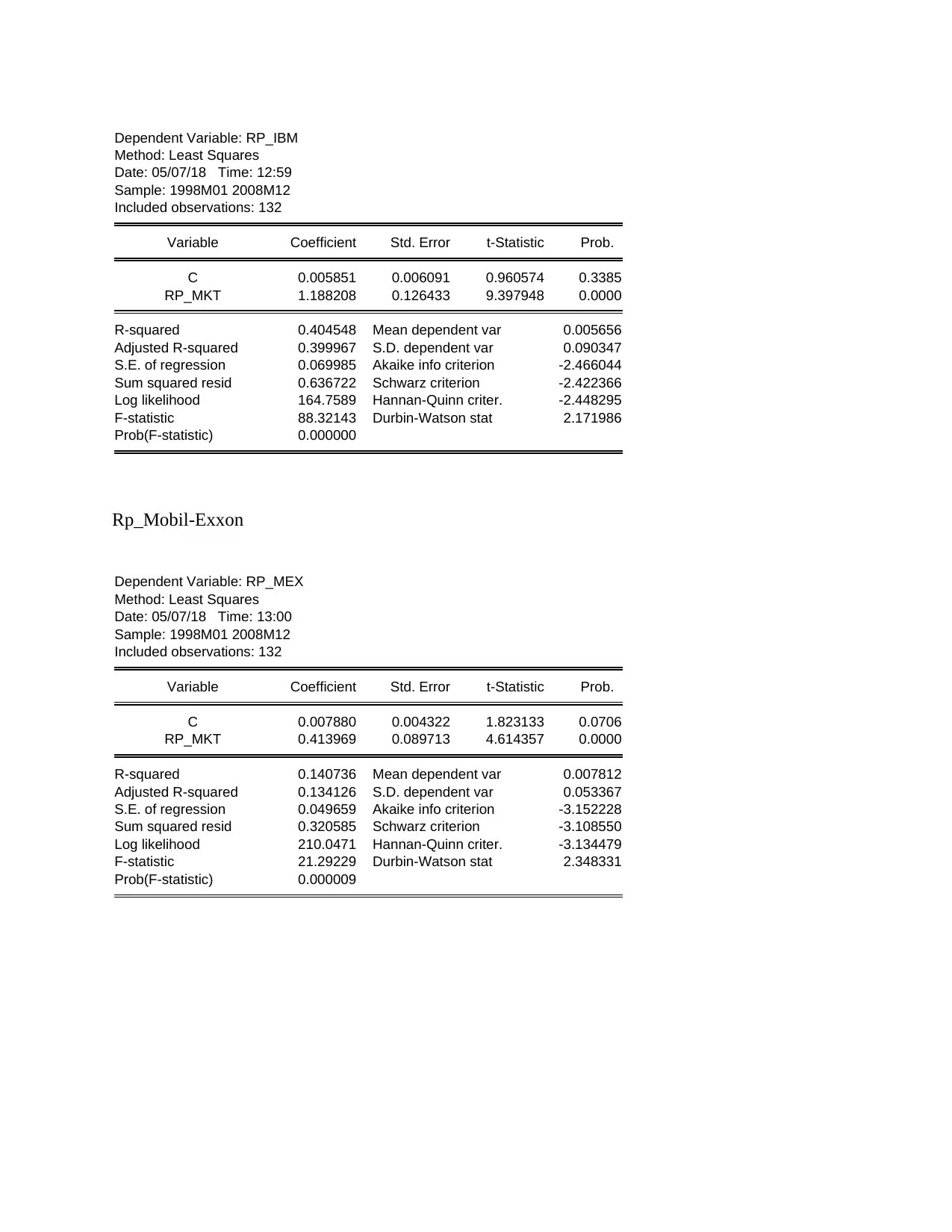
Rp_IBM

Dependent Variable: RP_IBM
Method: Least Squares
Date: 05/07/18 Time: 12:59
Sample: 1998M01 2008M12
Included observations: 132
Variable Coefficient Std. Error t-Statistic Prob.
C 0.005851 0.006091 0.960574 0.3385
RP_MKT 1.188208 0.126433 9.397948 0.0000
R-squared 0.404548 Mean dependent var 0.005656
Adjusted R-squared 0.399967 S.D. dependent var 0.090347
S.E. of regression 0.069985 Akaike info criterion -2.466044
Sum squared resid 0.636722 Schwarz criterion -2.422366
Log likelihood 164.7589 Hannan-Quinn criter. -2.448295
F-statistic 88.32143 Durbin-Watson stat 2.171986
Prob(F-statistic) 0.000000
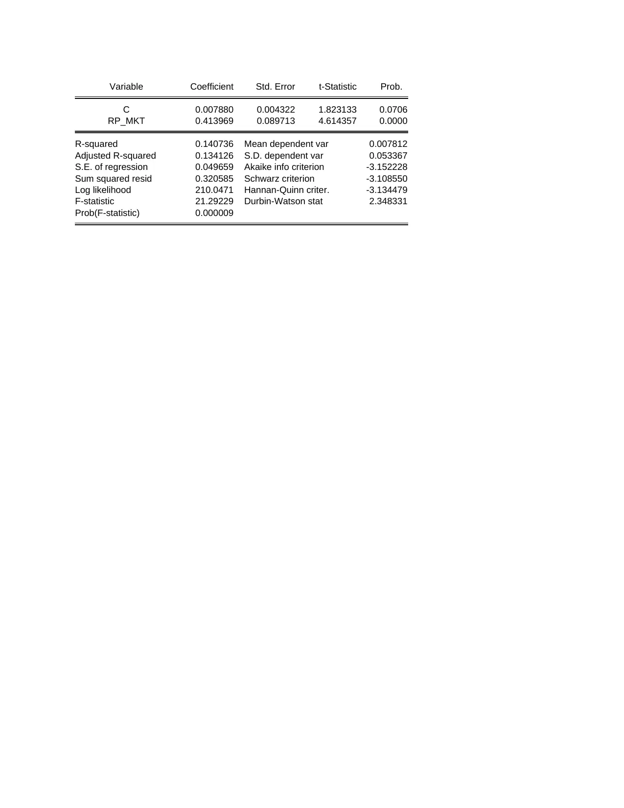
Rp_Mobil-Exxon
Dependent Variable: RP_MEX
Method: Least Squares
Date: 05/07/18 Time: 13:00
Sample: 1998M01 2008M12
Included observations: 132
Variable Coefficient Std. Error t-Statistic Prob.
C 0.007880 0.004322 1.823133 0.0706
RP_MKT 0.413969 0.089713 4.614357 0.0000
R-squared 0.140736 Mean dependent var 0.007812
Adjusted R-squared 0.134126 S.D. dependent var 0.053367
S.E. of regression 0.049659 Akaike info criterion -3.152228
Sum squared resid 0.320585 Schwarz criterion -3.108550
Log likelihood 210.0471 Hannan-Quinn criter. -3.134479
F-statistic 21.29229 Durbin-Watson stat 2.348331
Prob(F-statistic) 0.000009

APPENDIX
1.
Question 1
Dependent Variable: RP_MS
Method: Least Squares
Date: 05/07/18 Time: 11:59
Sample: 1998M01 2008M12
Included observations: 132
Variable Coefficient Std. Error t-Statistic Prob.
C 0.006098 0.007747 0.787109 0.4327
RP_MKT 1.318947 0.160790 8.202908 0.0000
R-squared 0.341064 Mean dependent var 0.005881
Adjusted R-squared 0.335995 S.D. dependent var 0.109224
S.E. of regression 0.089003 Akaike info criterion -1.985265
Sum squared resid 1.029792 Schwarz criterion -1.941586
Log likelihood 133.0275 Hannan-Quinn criter. -1.967516
F-statistic 67.28771 Durbin-Watson stat 2.345050
Prob(F-statistic) 0.000000
2.
Question 4
Wald Test:
Equation: Untitled
Test Statistic Value df Probability
t-statistic 8.202908 130 0.0000
F-statistic 67.28771 (1, 130) 0.0000
Chi-square 67.28771 1 0.0000
Null Hypothesis: C(2)=0
Null Hypothesis Summary:
Normalized Restriction (= 0) Value Std. Err.
C(2) 1.318947 0.160790
Restrictions are linear in coefficients.

3.
Question 8
Rp-Disney
Dependent Variable: RP_DISNEY
Method: Least Squares
Date: 05/07/18 Time: 12:56
Sample: 1998M01 2008M12
Included observations: 132
Variable Coefficient Std. Error t-Statistic Prob.
C -0.001149 0.005956 -0.192976 0.8473
RP_MKT 0.897838 0.123627 7.262477 0.0000
R-squared 0.288621 Mean dependent var -0.001297
Adjusted R-squared 0.283149 S.D. dependent var 0.080824
S.E. of regression 0.068432 Akaike info criterion -2.510928
Sum squared resid 0.608775 Schwarz criterion -2.467249
Log likelihood 167.7212 Hannan-Quinn criter. -2.493179
F-statistic 52.74358 Durbin-Watson stat 2.426356
Prob(F-statistic) 0.000000
Rp_GE
Dependent Variable: RP_GE
Method: Least Squares
Date: 05/07/18 Time: 12:58
Sample: 1998M01 2008M12
Included observations: 132
Variable Coefficient Std. Error t-Statistic Prob.
C -0.001167 0.004759 -0.245194 0.8067
RP_MKT 0.899260 0.098782 9.103512 0.0000
R-squared 0.389310 Mean dependent var -0.001314
Adjusted R-squared 0.384612 S.D. dependent var 0.069702
S.E. of regression 0.054679 Akaike info criterion -2.959642
Sum squared resid 0.388672 Schwarz criterion -2.915963
Log likelihood 197.3363 Hannan-Quinn criter. -2.941893
F-statistic 82.87393 Durbin-Watson stat 2.239423
Prob(F-statistic) 0.000000
Rp_GM

Dependent Variable: RP_GM
Method: Least Squares
Date: 05/07/18 Time: 12:58
Sample: 1998M01 2008M12
Included observations: 132
Variable Coefficient Std. Error t-Statistic Prob.
C -0.011550 0.009743 -1.185474 0.2380
RP_MKT 1.261411 0.202223 6.237709 0.0000
R-squared 0.230355 Mean dependent var -0.011757
Adjusted R-squared 0.224435 S.D. dependent var 0.127106
S.E. of regression 0.111937 Akaike info criterion -1.526719
Sum squared resid 1.628896 Schwarz criterion -1.483041
Log likelihood 102.7635 Hannan-Quinn criter. -1.508970
F-statistic 38.90901 Durbin-Watson stat 2.062907
Prob(F-statistic) 0.000000
Rp_IBM
Dependent Variable: RP_IBM
Method: Least Squares
Date: 05/07/18 Time: 12:59
Sample: 1998M01 2008M12
Included observations: 132
Variable Coefficient Std. Error t-Statistic Prob.
C 0.005851 0.006091 0.960574 0.3385
RP_MKT 1.188208 0.126433 9.397948 0.0000
R-squared 0.404548 Mean dependent var 0.005656
Adjusted R-squared 0.399967 S.D. dependent var 0.090347
S.E. of regression 0.069985 Akaike info criterion -2.466044
Sum squared resid 0.636722 Schwarz criterion -2.422366
Log likelihood 164.7589 Hannan-Quinn criter. -2.448295
F-statistic 88.32143 Durbin-Watson stat 2.171986
Prob(F-statistic) 0.000000
Rp_Mobil-Exxon
Dependent Variable: RP_MEX
Method: Least Squares
Date: 05/07/18 Time: 13:00
Sample: 1998M01 2008M12
Included observations: 132

Variable Coefficient Std. Error t-Statistic Prob.
C 0.007880 0.004322 1.823133 0.0706
RP_MKT 0.413969 0.089713 4.614357 0.0000
R-squared 0.140736 Mean dependent var 0.007812
Adjusted R-squared 0.134126 S.D. dependent var 0.053367
S.E. of regression 0.049659 Akaike info criterion -3.152228
Sum squared resid 0.320585 Schwarz criterion -3.108550
Log likelihood 210.0471 Hannan-Quinn criter. -3.134479
F-statistic 21.29229 Durbin-Watson stat 2.348331
Prob(F-statistic) 0.000009