Excel Assignment: Financial Analysis and Calculations Solutions

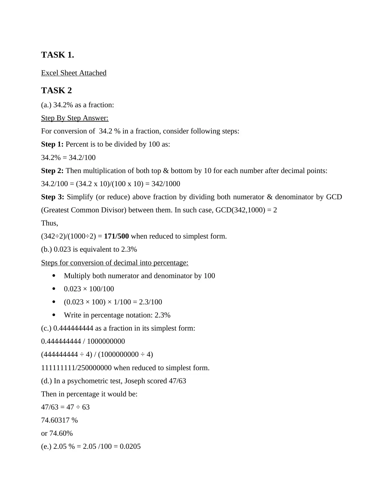
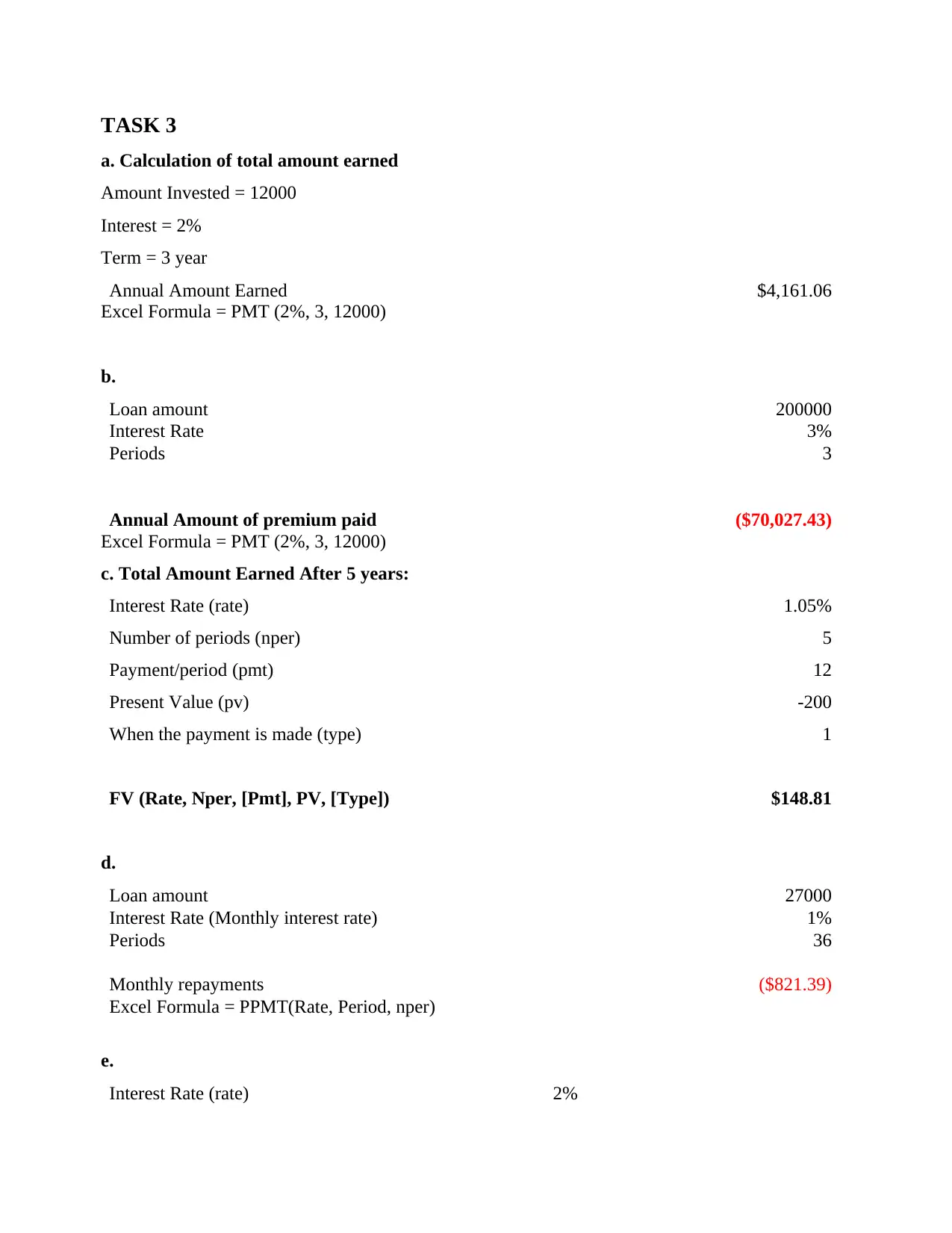
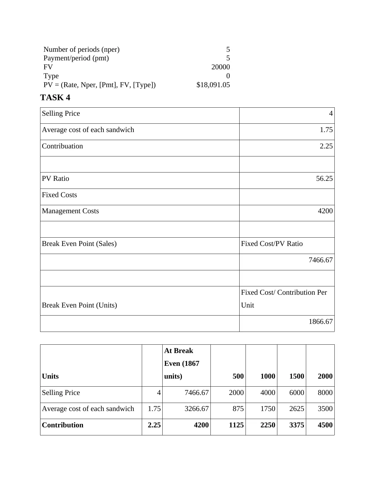
This document presents a comprehensive solution to an Excel-based finance assignment. It covers a range of financial calculations, including percentage conversions, loan and investment calculations using formulas like PMT, and break-even point analysis. The assignment also includes data analysi...Read More

Excel Questions

Table of Contents
TASK 1............................................................................................................................................3
Excel Sheet Attached..............................................................................................................3
TASK 2............................................................................................................................................3
TASK 3............................................................................................................................................4
TASK 4............................................................................................................................................5
TASK 5............................................................................................................................................6

TASK 1.
Excel Sheet Attached
TASK 2
(a.) 34.2% as a fraction:
Step By Step Answer:
For conversion of 34.2 % in a fraction, consider following steps:
Step 1: Percent is to be divided by 100 as:
34.2% = 34.2/100
Step 2: Then multiplication of both top & bottom by 10 for each number after decimal points:
34.2/100 = (34.2 x 10)/(100 x 10) = 342/1000
Step 3: Simplify (or reduce) above fraction by dividing both numerator & denominator by GCD
(Greatest Common Divisor) between them. In such case, GCD(342,1000) = 2
Thus,
(342÷2)/(1000÷2) = 171/500 when reduced to simplest form.
(b.) 0.023 is equivalent to 2.3%
Steps for conversion of decimal into percentage:
 Multiply both numerator and denominator by 100
 0.023 × 100/100
 (0.023 × 100) × 1/100 = 2.3/100
 Write in percentage notation: 2.3%
(c.) 0.444444444 as a fraction in its simplest form:
0.444444444 / 1000000000
(444444444 ÷ 4) / (1000000000 ÷ 4)
111111111/250000000 when reduced to simplest form.
(d.) In a psychometric test, Joseph scored 47/63
Then in percentage it would be:
47/63 = 47 ÷ 63
74.60317 %
or 74.60%
(e.) 2.05 % = 2.05 /100 = 0.0205

TASK 3
a. Calculation of total amount earned
Amount Invested = 12000
Interest = 2%
Term = 3 year
Annual Amount Earned $4,161.06
Excel Formula = PMT (2%, 3, 12000)
b.
Loan amount 200000
Interest Rate 3%
Periods 3
Annual Amount of premium paid ($70,027.43)
Excel Formula = PMT (2%, 3, 12000)
c. Total Amount Earned After 5 years:
Interest Rate (rate) 1.05%
Number of periods (nper) 5
Payment/period (pmt) 12
Present Value (pv) -200
When the payment is made (type) 1
FV (Rate, Nper, [Pmt], PV, [Type]) $148.81
d.
Loan amount 27000
Interest Rate (Monthly interest rate) 1%
Periods 36
Monthly repayments ($821.39)
Excel Formula = PPMT(Rate, Period, nper)
e.
Interest Rate (rate) 2%

Number of periods (nper) 5
Payment/period (pmt) 5
FV 20000
Type 0
PV = (Rate, Nper, [Pmt], FV, [Type]) $18,091.05
TASK 4
Selling Price 4
Average cost of each sandwich 1.75
Contribuation 2.25
PV Ratio 56.25
Fixed Costs
Management Costs 4200
Break Even Point (Sales) Fixed Cost/PV Ratio
7466.67
Break Even Point (Units)
Fixed Cost/ Contribution Per
Unit
1866.67
Units
At Break
Even (1867
units) 500 1000 1500 2000
Selling Price 4 7466.67 2000 4000 6000 8000
Average cost of each sandwich 1.75 3266.67 875 1750 2625 3500
Contribution 2.25 4200 1125 2250 3375 4500

Fixed Costs
Management Costs 4200 4200 4200 4200 4200 4200
Net Profit/(Loss) 0 -3075 -1950 -825 300

TASK 5
Employees Number of Leaves
1 6
2 12
3 12
4 14
5 6
6 14
7 12
8 9
9 12
10 11
11 12
12 12
13 7
14 12
15 17
16 14
17 13
18 12
19 13
20 12
21 12
22 12

a. 18 Employees
=COUNTIF(number of leave,">10")
b. 11 Employees
=COUNTIF(number of trainings,"<2")
c.
=IF(AND(number of leave,">10",number of trainings,"<2"),"YES","NO")
Employees Number of Leaves Number of days training
1 6 1 NO
2 12 2 YES
3 12 1 YES
4 14 1 YES
5 6 4 NO
6 14 1 YES
7 12 2 YES
8 9 2 NO
9 12 1 YES
10 11 1 YES
11 12 1 YES
12 12 2 YES
13 7 2 NO
14 12 3 NO
15 17 3 NO
16 14 1 YES
17 13 1 YES
18 12 2 YES

19 13 1 YES
20 12 1 YES
21 12 2 YES
22 12 4 NO