Economics Assignment: Expenditure Multiplier and Economic Analysis
VerifiedAdded on 2023/03/29
|8
|1424
|257
Homework Assignment
AI Summary
This economics assignment provides a comprehensive overview of the expenditure multiplier, explaining its impact on economic activity and the circular flow of expenditure. It defines key economic indicators like GDP and NDP. The assignment then delves into fiscal and monetary policies, illustrating their effects with diagrams. It also covers various types of unemployment, demand-pull and cost-push inflation, and the application of aggregate demand and supply to economic situations. Furthermore, the assignment explains cost reconciliation, cost curves (fixed, variable, and total), production possibility frontiers, and profit maximization determination. The assignment uses diagrams and references to support the concepts discussed, offering a well-rounded analysis of core economic principles.
Expenditure multiplier application
In simple words, expenditure multiplier said to be in play when an investment fell by $100
billion, its impact on an economy not remain only limited $ 100 billion, in fact, its impact felt
many times more than $ 100 billion that is what multiplier mean. It can be 2 times, 3 times or
even 5 times, it depends on multiplier number. Investment or expenditure can be of many
types, it can be consumption, investment, Government expenditure or net of exports and
imports, its impact on an economy have more than proportional change in expenditure or
investment. (Ceteris paribus) This is what multiplier mean for an economy. As per the
Keynsean economics, higher the aggregate demand, higher will be economic activity.
Aggregate expenditure circulates in an economy: that is popularly known as circular flow of
expenditure/income in an economy. It works like this, households buy from firms, firms pay
workers and suppliers, workers and suppliers buy goods from other firms, those firms pay
their workers and suppliers, and so on so forth. In this way original expenditure converted to
many time through the impact of multiplier, this is what expenditure multiplier mean.
GDP (Gross Domestic Product):
Monetary value of final (not intermediate) Goods and Services produced in an economy
(domestic territory) in a financial year.
GDP = C + I + G + (X – M) = Private consumption + gross consumption +
government spending + (export-imports)
NDP (Net Domestic Product):
NDP = GDP - Depreciation or (wear and tear)
Fiscal Policy and Monetary policy with diagram
(ceteris paribus applicable wherever it is required)
Fiscal policy is implemented by government of that country: It is done by influencing
investment, employment, output and income, (ceteris paribus) through following two ways:
a) Increase/decrease in expenditure and
Paraphrase This Document
Need a fresh take? Get an instant paraphrase of this document with our AI Paraphraser
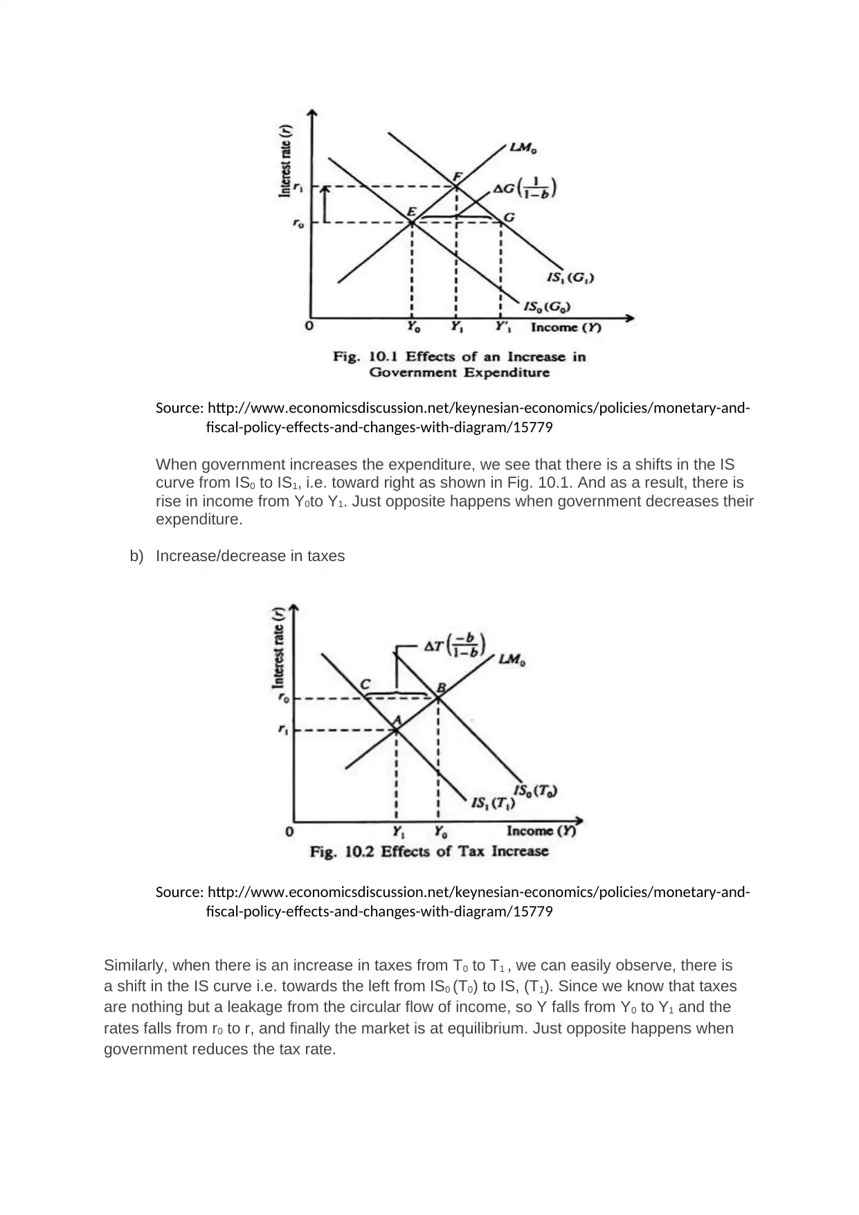
Source: http://www.economicsdiscussion.net/keynesian-economics/policies/monetary-and-
fiscal-policy-effects-and-changes-with-diagram/15779
When government increases the expenditure, we see that there is a shifts in the IS
curve from IS0 to IS1, i.e. toward right as shown in Fig. 10.1. And as a result, there is
rise in income from Y0to Y1. Just opposite happens when government decreases their
expenditure.
b) Increase/decrease in taxes
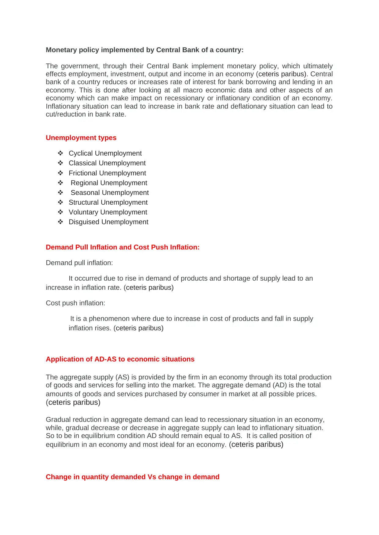
Source: http://www.economicsdiscussion.net/keynesian-economics/policies/monetary-and-
fiscal-policy-effects-and-changes-with-diagram/15779
Similarly, when there is an increase in taxes from T0 to T1 , we can easily observe, there is
a shift in the IS curve i.e. towards the left from IS0 (T0) to IS, (T1). Since we know that taxes
are nothing but a leakage from the circular flow of income, so Y falls from Y0 to Y1 and the
rates falls from r0 to r, and finally the market is at equilibrium. Just opposite happens when
government reduces the tax rate.
fiscal-policy-effects-and-changes-with-diagram/15779
When government increases the expenditure, we see that there is a shifts in the IS
curve from IS0 to IS1, i.e. toward right as shown in Fig. 10.1. And as a result, there is
rise in income from Y0to Y1. Just opposite happens when government decreases their
expenditure.
b) Increase/decrease in taxes
Source: http://www.economicsdiscussion.net/keynesian-economics/policies/monetary-and-
fiscal-policy-effects-and-changes-with-diagram/15779
Similarly, when there is an increase in taxes from T0 to T1 , we can easily observe, there is
a shift in the IS curve i.e. towards the left from IS0 (T0) to IS, (T1). Since we know that taxes
are nothing but a leakage from the circular flow of income, so Y falls from Y0 to Y1 and the
rates falls from r0 to r, and finally the market is at equilibrium. Just opposite happens when
government reduces the tax rate.
Monetary policy implemented by Central Bank of a country:
The government, through their Central Bank implement monetary policy, which ultimately
effects employment, investment, output and income in an economy (ceteris paribus). Central
bank of a country reduces or increases rate of interest for bank borrowing and lending in an
economy. This is done after looking at all macro economic data and other aspects of an
economy which can make impact on recessionary or inflationary condition of an economy.
Inflationary situation can lead to increase in bank rate and deflationary situation can lead to
cut/reduction in bank rate.
Unemployment types
Cyclical Unemployment
Classical Unemployment
Frictional Unemployment
Regional Unemployment
Seasonal Unemployment
Structural Unemployment
Voluntary Unemployment
Disguised Unemployment
Demand Pull Inflation and Cost Push Inflation:
Demand pull inflation:
It occurred due to rise in demand of products and shortage of supply lead to an
increase in inflation rate. (ceteris paribus)
Cost push inflation:
It is a phenomenon where due to increase in cost of products and fall in supply
inflation rises. (ceteris paribus)
Application of AD-AS to economic situations
The aggregate supply (AS) is provided by the firm in an economy through its total production
of goods and services for selling into the market. The aggregate demand (AD) is the total
amounts of goods and services purchased by consumer in market at all possible prices.
(ceteris paribus)
Gradual reduction in aggregate demand can lead to recessionary situation in an economy,
while, gradual decrease or decrease in aggregate supply can lead to inflationary situation.
So to be in equilibrium condition AD should remain equal to AS. It is called position of
equilibrium in an economy and most ideal for an economy. (ceteris paribus)
Change in quantity demanded Vs change in demand
⊘ This is a preview!⊘
Do you want full access?
Subscribe today to unlock all pages.

Trusted by 1+ million students worldwide
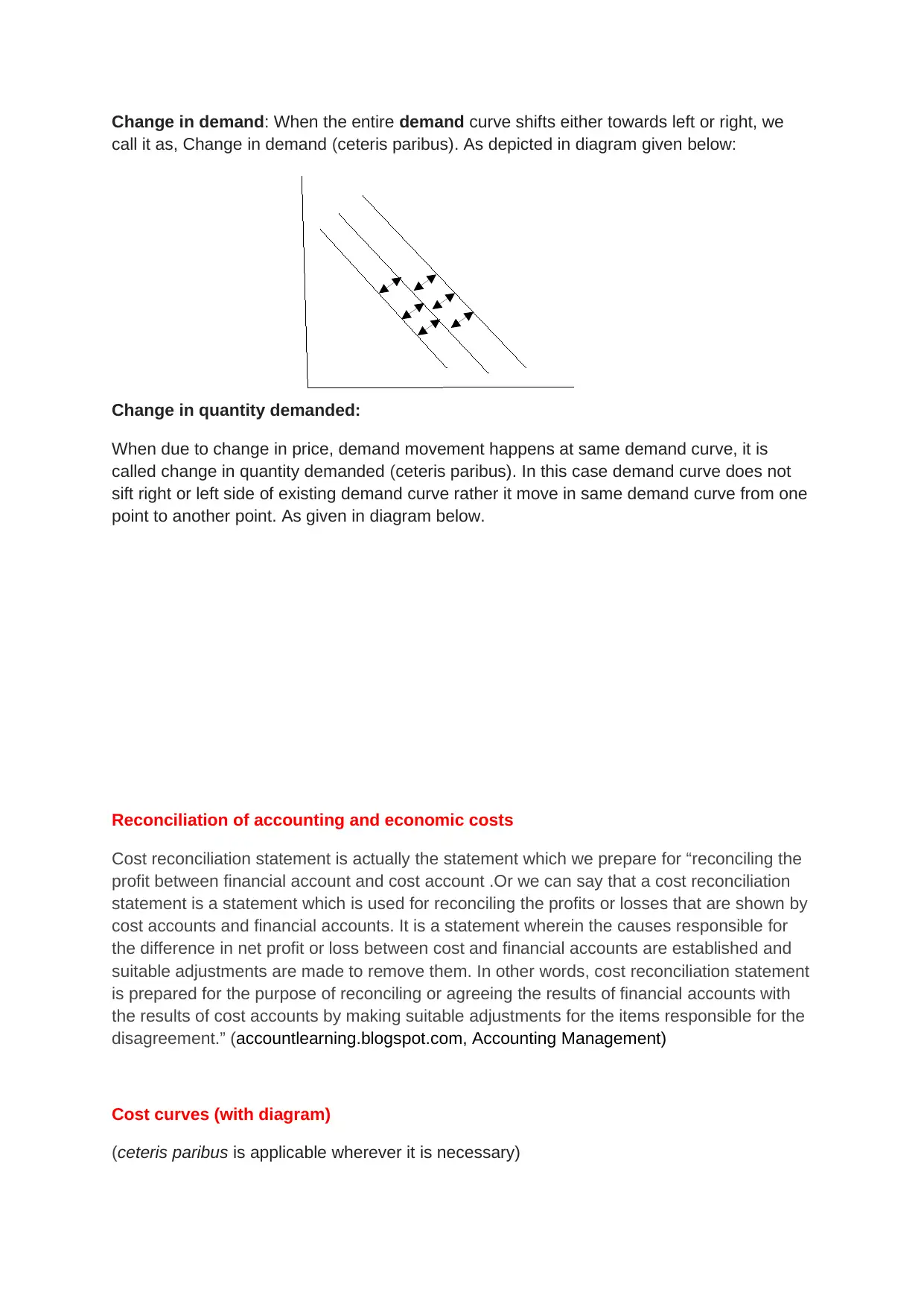
Change in demand: When the entire demand curve shifts either towards left or right, we
call it as, Change in demand (ceteris paribus). As depicted in diagram given below:
Change in quantity demanded:
When due to change in price, demand movement happens at same demand curve, it is
called change in quantity demanded (ceteris paribus). In this case demand curve does not
sift right or left side of existing demand curve rather it move in same demand curve from one
point to another point. As given in diagram below.
Reconciliation of accounting and economic costs
Cost reconciliation statement is actually the statement which we prepare for “reconciling the
profit between financial account and cost account .Or we can say that a cost reconciliation
statement is a statement which is used for reconciling the profits or losses that are shown by
cost accounts and financial accounts. It is a statement wherein the causes responsible for
the difference in net profit or loss between cost and financial accounts are established and
suitable adjustments are made to remove them. In other words, cost reconciliation statement
is prepared for the purpose of reconciling or agreeing the results of financial accounts with
the results of cost accounts by making suitable adjustments for the items responsible for the
disagreement.” (accountlearning.blogspot.com, Accounting Management)
Cost curves (with diagram)
(ceteris paribus is applicable wherever it is necessary)
Paraphrase This Document
Need a fresh take? Get an instant paraphrase of this document with our AI Paraphraser
Fixed cost:
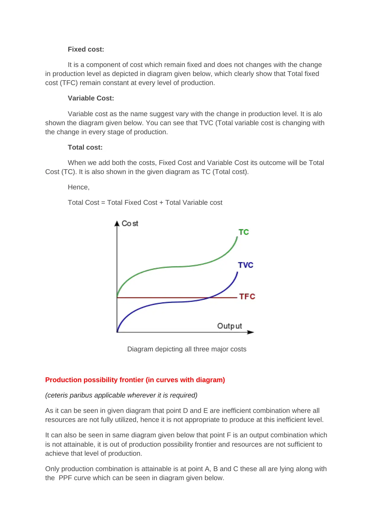
It is a component of cost which remain fixed and does not changes with the change
in production level as depicted in diagram given below, which clearly show that Total fixed
cost (TFC) remain constant at every level of production.
Variable Cost:
Variable cost as the name suggest vary with the change in production level. It is alo
shown the diagram given below. You can see that TVC (Total variable cost is changing with
the change in every stage of production.
Total cost:
When we add both the costs, Fixed Cost and Variable Cost its outcome will be Total
Cost (TC). It is also shown in the given diagram as TC (Total cost).
Hence,
Total Cost = Total Fixed Cost + Total Variable cost
Diagram depicting all three major costs
Production possibility frontier (in curves with diagram)
(ceteris paribus applicable wherever it is required)
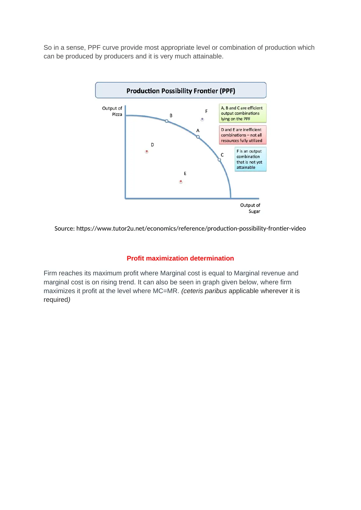
As it can be seen in given diagram that point D and E are inefficient combination where all
resources are not fully utilized, hence it is not appropriate to produce at this inefficient level.
It can also be seen in same diagram given below that point F is an output combination which
is not attainable, it is out of production possibility frontier and resources are not sufficient to
achieve that level of production.
Only production combination is attainable is at point A, B and C these all are lying along with
the PPF curve which can be seen in diagram given below.
So in a sense, PPF curve provide most appropriate level or combination of production which
can be produced by producers and it is very much attainable.
Source: https://www.tutor2u.net/economics/reference/production-possibility-frontier-video
Profit maximization determination
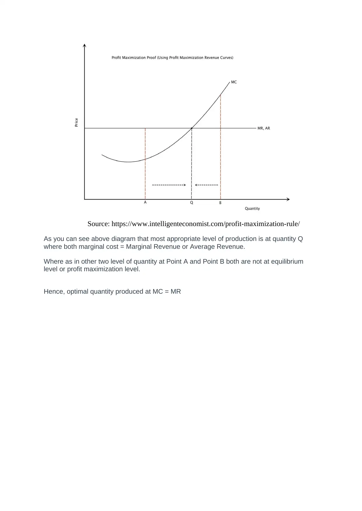
Firm reaches its maximum profit where Marginal cost is equal to Marginal revenue and
marginal cost is on rising trend. It can also be seen in graph given below, where firm
maximizes it profit at the level where MC=MR. (ceteris paribus applicable wherever it is
required)
⊘ This is a preview!⊘
Do you want full access?
Subscribe today to unlock all pages.

Trusted by 1+ million students worldwide
Source: https://www.intelligenteconomist.com/profit-maximization-rule/
As you can see above diagram that most appropriate level of production is at quantity Q
where both marginal cost = Marginal Revenue or Average Revenue.
Where as in other two level of quantity at Point A and Point B both are not at equilibrium
level or profit maximization level.
Hence, optimal quantity produced at MC = MR
Paraphrase This Document
Need a fresh take? Get an instant paraphrase of this document with our AI Paraphraser
References:
courses.lumenlearning.com, The Expenditure Multiplier Effect. Retrieved June 06, 2019, From
https://courses.lumenlearning.com/wm-macroeconomics/chapter/the-expenditure-multiplier-effect/
accountlearning.blogspot.com, Accounting Management. Retrieved June 06, 2019, From
https://accountlearning.blogspot.com/2011/12/concept-and-meaning-of-cost.html
Kari, Diptimai, Monetary and Fiscal Policy: Effects and Changes (With Diagram). Retrieved June 06,
2019, From http://www.economicsdiscussion.net/keynesian-economics/policies/monetary-and-fiscal-
policy-effects-and-changes-with-diagram/15779
Chand, Smriti, Effectiveness of Monetary and Fiscal Policy (explained with diagram). Retrieved June
06, 2019, From http://www.yourarticlelibrary.com/policies/effectiveness-of-monetary-and-fiscal-policy-
explained-with-diagram-economics/29271
Boundless Economics, Introducing Aggregate Demand and Aggregate Supply. Retrieved June 06,
2019, From https://courses.lumenlearning.com/boundless-economics/chapter/introducing-aggregate-
demand-and-aggregate-supply/
Intelligent Economist, (2019). Profit Maximization Rule. Retrieved June 06, 2019, From
https://www.intelligenteconomist.com/profit-maximization-rule/
1 out of 8
Related Documents
Your All-in-One AI-Powered Toolkit for Academic Success.
+13062052269
info@desklib.com
Available 24*7 on WhatsApp / Email
![[object Object]](/_next/static/media/star-bottom.7253800d.svg)
Unlock your academic potential
Copyright © 2020–2026 A2Z Services. All Rights Reserved. Developed and managed by ZUCOL.


