Exploratory Functional Analysis and Cluster Analysis with R
VerifiedAdded on 2023/05/30
|18
|2141
|171
AI Summary
This article discusses exploratory factor analysis, Cronbach alpha, correlation output, hierarchical clustering, and partition clustering with R. It also highlights the differences between expert and amateur sensometric ratings. The article analyzes the distance matrix data for Asian continent using clustering techniques. The article is relevant for students studying data analysis and statistics. The course code, course name, and college/university are not mentioned.
Contribute Materials
Your contribution can guide someone’s learning journey. Share your
documents today.

1
Exploratory Functional Analysis and
Cluster Analysis with R
Exploratory Functional Analysis and
Cluster Analysis with R
Secure Best Marks with AI Grader
Need help grading? Try our AI Grader for instant feedback on your assignments.
2
Question 1
Initial Data Discussion
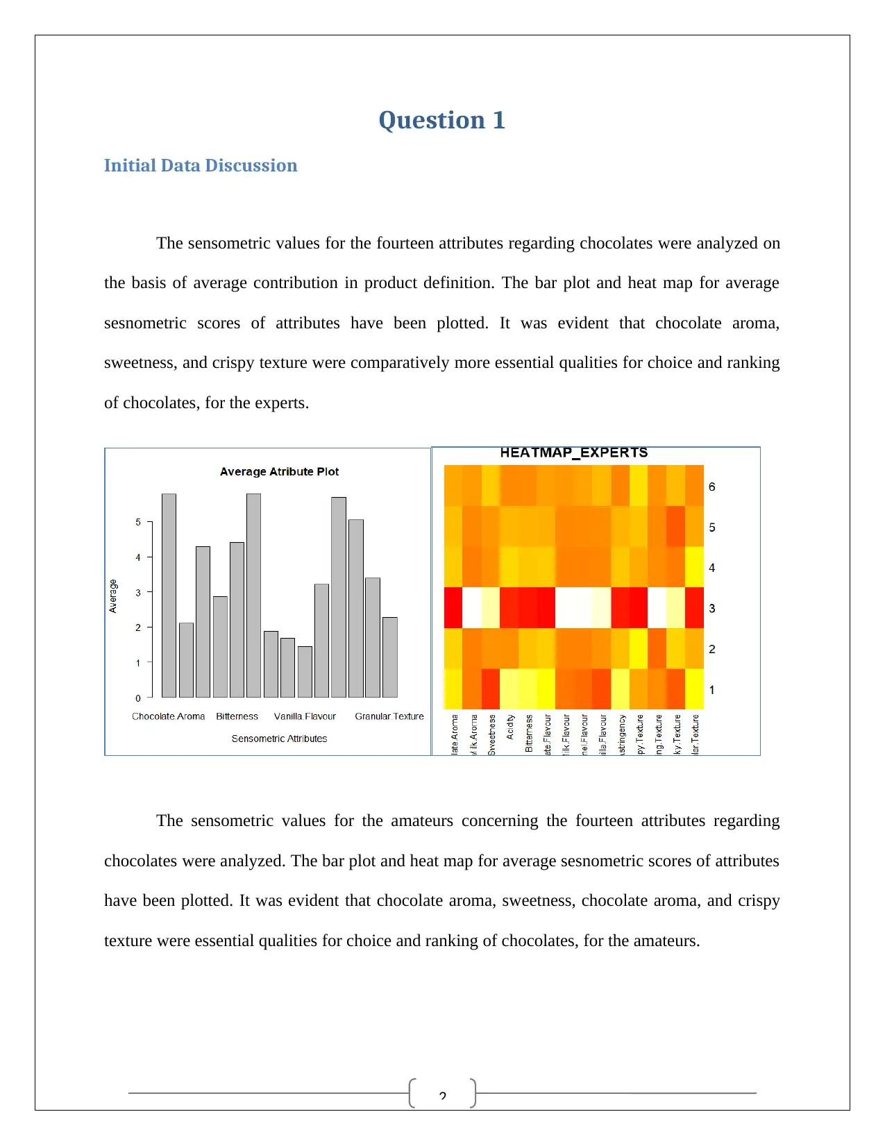
The sensometric values for the fourteen attributes regarding chocolates were analyzed on
the basis of average contribution in product definition. The bar plot and heat map for average
sesnometric scores of attributes have been plotted. It was evident that chocolate aroma,
sweetness, and crispy texture were comparatively more essential qualities for choice and ranking
of chocolates, for the experts.
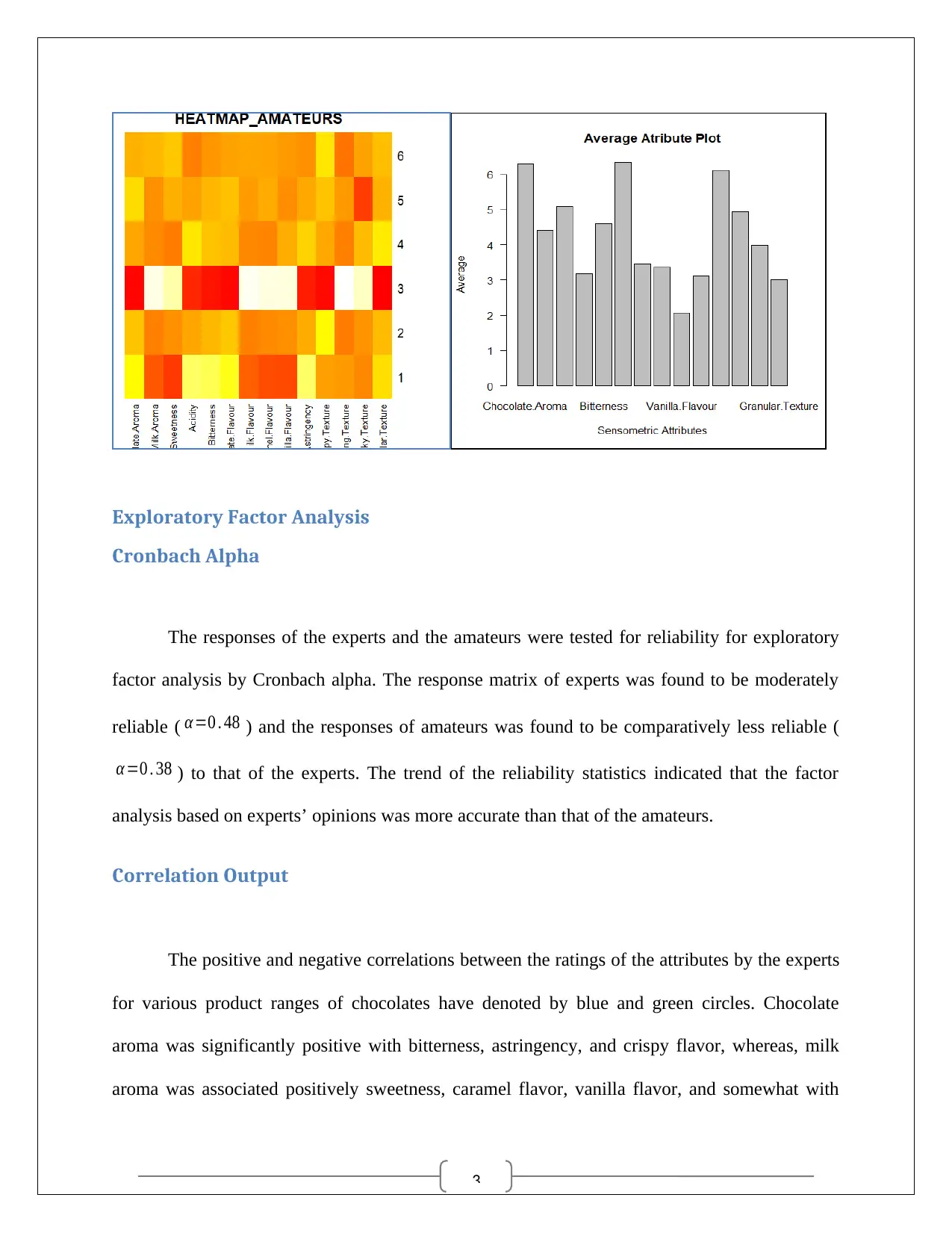
The sensometric values for the amateurs concerning the fourteen attributes regarding
chocolates were analyzed. The bar plot and heat map for average sesnometric scores of attributes
have been plotted. It was evident that chocolate aroma, sweetness, chocolate aroma, and crispy
texture were essential qualities for choice and ranking of chocolates, for the amateurs.
Question 1
Initial Data Discussion
The sensometric values for the fourteen attributes regarding chocolates were analyzed on
the basis of average contribution in product definition. The bar plot and heat map for average
sesnometric scores of attributes have been plotted. It was evident that chocolate aroma,
sweetness, and crispy texture were comparatively more essential qualities for choice and ranking
of chocolates, for the experts.
The sensometric values for the amateurs concerning the fourteen attributes regarding
chocolates were analyzed. The bar plot and heat map for average sesnometric scores of attributes
have been plotted. It was evident that chocolate aroma, sweetness, chocolate aroma, and crispy
texture were essential qualities for choice and ranking of chocolates, for the amateurs.
3
Exploratory Factor Analysis
Cronbach Alpha
The responses of the experts and the amateurs were tested for reliability for exploratory
factor analysis by Cronbach alpha. The response matrix of experts was found to be moderately
reliable ( α=0 . 48 ) and the responses of amateurs was found to be comparatively less reliable (
α =0 . 38 ) to that of the experts. The trend of the reliability statistics indicated that the factor
analysis based on experts’ opinions was more accurate than that of the amateurs.
Correlation Output
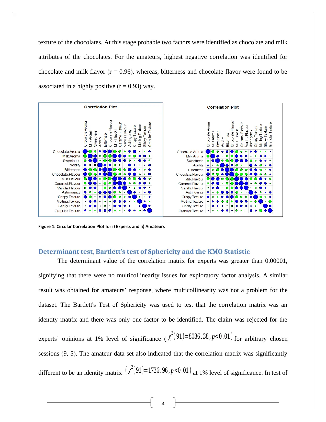
The positive and negative correlations between the ratings of the attributes by the experts
for various product ranges of chocolates have denoted by blue and green circles. Chocolate
aroma was significantly positive with bitterness, astringency, and crispy flavor, whereas, milk
aroma was associated positively sweetness, caramel flavor, vanilla flavor, and somewhat with
Exploratory Factor Analysis
Cronbach Alpha
The responses of the experts and the amateurs were tested for reliability for exploratory
factor analysis by Cronbach alpha. The response matrix of experts was found to be moderately
reliable ( α=0 . 48 ) and the responses of amateurs was found to be comparatively less reliable (
α =0 . 38 ) to that of the experts. The trend of the reliability statistics indicated that the factor
analysis based on experts’ opinions was more accurate than that of the amateurs.
Correlation Output
The positive and negative correlations between the ratings of the attributes by the experts
for various product ranges of chocolates have denoted by blue and green circles. Chocolate
aroma was significantly positive with bitterness, astringency, and crispy flavor, whereas, milk
aroma was associated positively sweetness, caramel flavor, vanilla flavor, and somewhat with
4
texture of the chocolates. At this stage probable two factors were identified as chocolate and milk
attributes of the chocolates. For the amateurs, highest negative correlation was identified for
chocolate and milk flavor (r = 0.96), whereas, bitterness and chocolate flavor were found to be
associated in a highly positive (r = 0.93) way.
Figure 1: Circular Correlation Plot for i) Experts and ii) Amateurs
Determinant test, Bartlett’s test of Sphericity and the KMO Statistic
The determinant value of the correlation matrix for experts was greater than 0.00001,
signifying that there were no multicollinearity issues for exploratory factor analysis. A similar
result was obtained for amateurs’ response, where multicollinearity was not a problem for the
dataset. The Bartlett's Test of Sphericity was used to test that the correlation matrix was an
identity matrix and there was only one factor to be identified. The claim was rejected for the
experts’ opinions at 1% level of significance ( χ2( 91)=8086 . 38 , p< 0 .01 ) for arbitrary chosen
sessions (9, 5). The amateur data set also indicated that the correlation matrix was significantly
different to be an identity matrix ( χ2( 91)=1736 . 96 , p <0 .01 ) at 1% level of significance. In test of
Secure Best Marks with AI Grader
Need help grading? Try our AI Grader for instant feedback on your assignments.
5
adequacy of the sample data, Kaiser-Meyer-Olkin statistic was used, and the value was found to
be closer to 1 (KMO = 0.91). This signified that the sample dataset was adequate for factor
extraction. Parallel study for adequacy in amateur data revealed that (KMO = 0.83) there was
enough data for factor analysis.
Number of Factors to Estimate
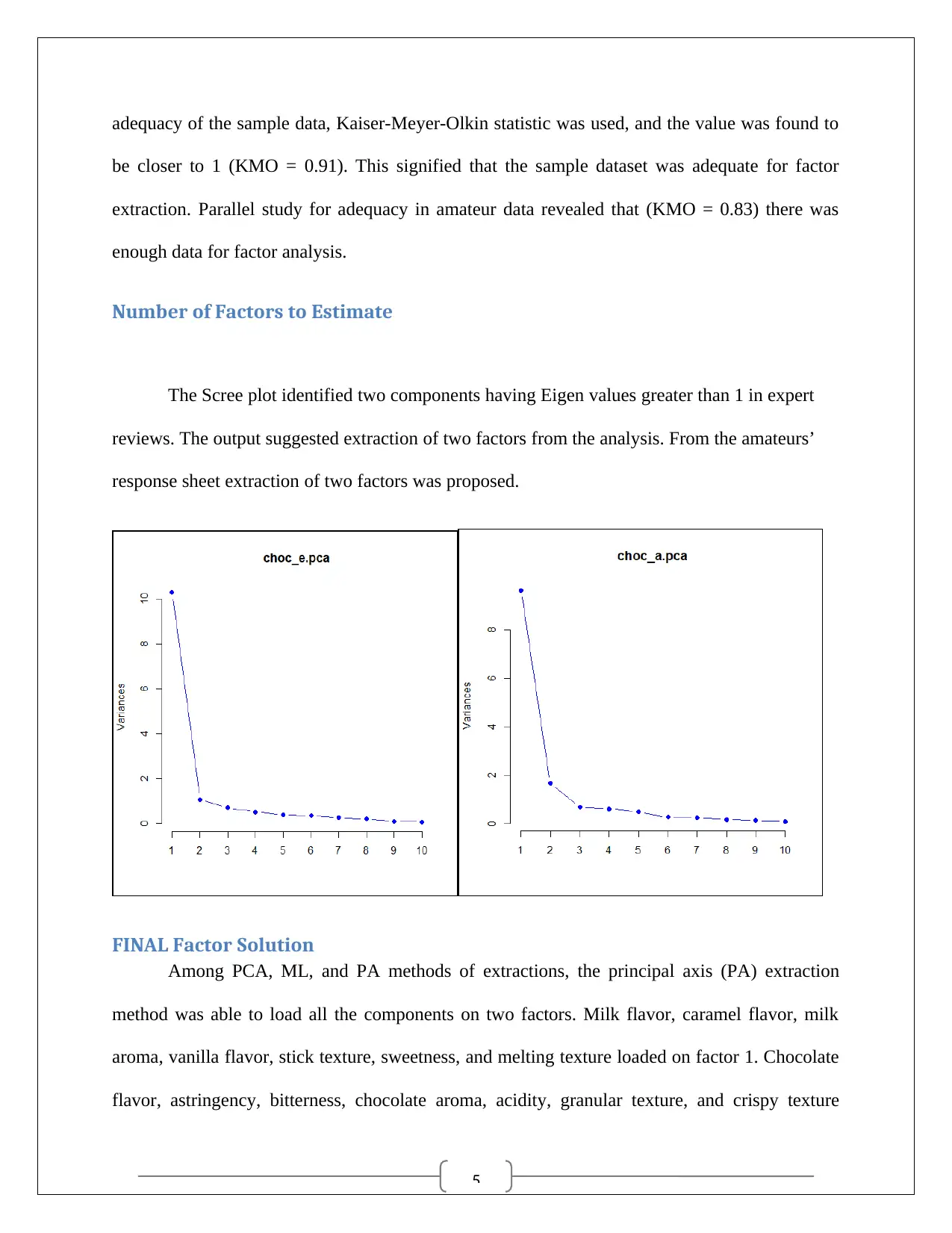
The Scree plot identified two components having Eigen values greater than 1 in expert
reviews. The output suggested extraction of two factors from the analysis. From the amateurs’
response sheet extraction of two factors was proposed.
FINAL Factor Solution
Among PCA, ML, and PA methods of extractions, the principal axis (PA) extraction
method was able to load all the components on two factors. Milk flavor, caramel flavor, milk
aroma, vanilla flavor, stick texture, sweetness, and melting texture loaded on factor 1. Chocolate
flavor, astringency, bitterness, chocolate aroma, acidity, granular texture, and crispy texture
adequacy of the sample data, Kaiser-Meyer-Olkin statistic was used, and the value was found to
be closer to 1 (KMO = 0.91). This signified that the sample dataset was adequate for factor
extraction. Parallel study for adequacy in amateur data revealed that (KMO = 0.83) there was
enough data for factor analysis.
Number of Factors to Estimate
The Scree plot identified two components having Eigen values greater than 1 in expert
reviews. The output suggested extraction of two factors from the analysis. From the amateurs’
response sheet extraction of two factors was proposed.
FINAL Factor Solution
Among PCA, ML, and PA methods of extractions, the principal axis (PA) extraction
method was able to load all the components on two factors. Milk flavor, caramel flavor, milk
aroma, vanilla flavor, stick texture, sweetness, and melting texture loaded on factor 1. Chocolate
flavor, astringency, bitterness, chocolate aroma, acidity, granular texture, and crispy texture
6
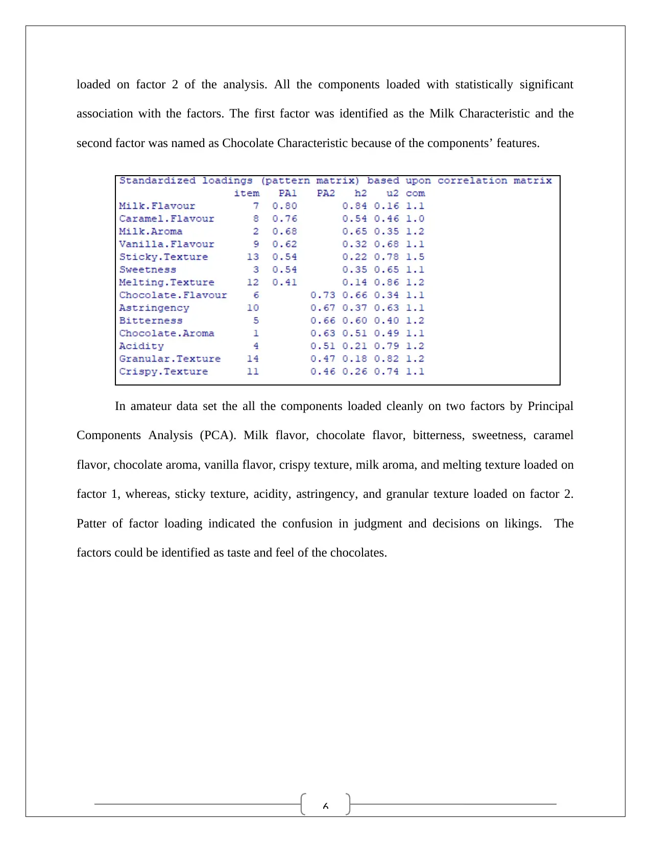
loaded on factor 2 of the analysis. All the components loaded with statistically significant
association with the factors. The first factor was identified as the Milk Characteristic and the
second factor was named as Chocolate Characteristic because of the components’ features.
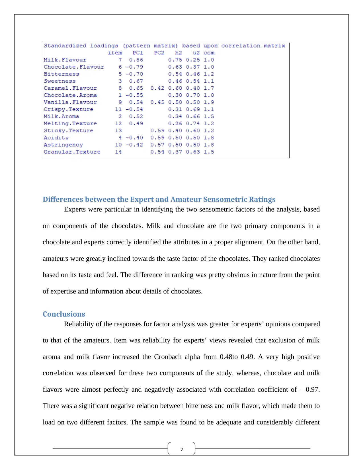
In amateur data set the all the components loaded cleanly on two factors by Principal
Components Analysis (PCA). Milk flavor, chocolate flavor, bitterness, sweetness, caramel
flavor, chocolate aroma, vanilla flavor, crispy texture, milk aroma, and melting texture loaded on
factor 1, whereas, sticky texture, acidity, astringency, and granular texture loaded on factor 2.
Patter of factor loading indicated the confusion in judgment and decisions on likings. The
factors could be identified as taste and feel of the chocolates.
loaded on factor 2 of the analysis. All the components loaded with statistically significant
association with the factors. The first factor was identified as the Milk Characteristic and the
second factor was named as Chocolate Characteristic because of the components’ features.
In amateur data set the all the components loaded cleanly on two factors by Principal
Components Analysis (PCA). Milk flavor, chocolate flavor, bitterness, sweetness, caramel
flavor, chocolate aroma, vanilla flavor, crispy texture, milk aroma, and melting texture loaded on
factor 1, whereas, sticky texture, acidity, astringency, and granular texture loaded on factor 2.
Patter of factor loading indicated the confusion in judgment and decisions on likings. The
factors could be identified as taste and feel of the chocolates.
7
Differences between the Expert and Amateur Sensometric Ratings
Experts were particular in identifying the two sensometric factors of the analysis, based
on components of the chocolates. Milk and chocolate are the two primary components in a
chocolate and experts correctly identified the attributes in a proper alignment. On the other hand,
amateurs were greatly inclined towards the taste factor of the chocolates. They ranked chocolates
based on its taste and feel. The difference in ranking was pretty obvious in nature from the point
of expertise and information about details of chocolates.
Conclusions
Reliability of the responses for factor analysis was greater for experts’ opinions compared
to that of the amateurs. Item was reliability for experts’ views revealed that exclusion of milk
aroma and milk flavor increased the Cronbach alpha from 0.48to 0.49. A very high positive
correlation was observed for these two components of the study, whereas, chocolate and milk
flavors were almost perfectly and negatively associated with correlation coefficient of – 0.97.
There was a significant negative relation between bitterness and milk flavor, which made them to
load on two different factors. The sample was found to be adequate and considerably different
Paraphrase This Document
Need a fresh take? Get an instant paraphrase of this document with our AI Paraphraser
8
from unit matrix for accurate factor extraction. Individual KMO statistics were significantly
high; the minimum value of 0.834 was noted for milk flavor of a chocolate. Sample size was
found to be sufficiently large for proper EFA.
Reliability for amateurs was found to be α= 0.38, which was found to increase up to 0.4
for removal of chocolate and milk flavor from the dataset. The most important aspect was
identified as the sticky texture, and astringency of the chocolates. Caramel flavor was the
dominant reason for reliability purpose. Here, chocolate flavor and bitterness had highly positive
correlation, whereas relation between chocolate and milk flavor, and sweetness and bitterness
were highly negative. The sample was found to be adequate and considerably different from unit
matrix for accurate factor extraction. Individual KMO statistics were significantly high; the
minimum value of 0.834 was noted for milk flavor of a chocolate. Sample size was found to be
large for EFA. The preference for ranking the chocolates was solely based on taste and feel of
the chocolate. From the correlation between the factors, it was noted that no oblique rotation was
required for EFA (Hanna, de Araújo, Vilarino, & Mayhew, 2016).
9
Question 2
Initial Data Discussion
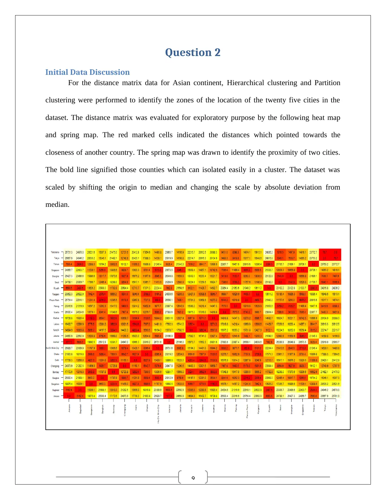
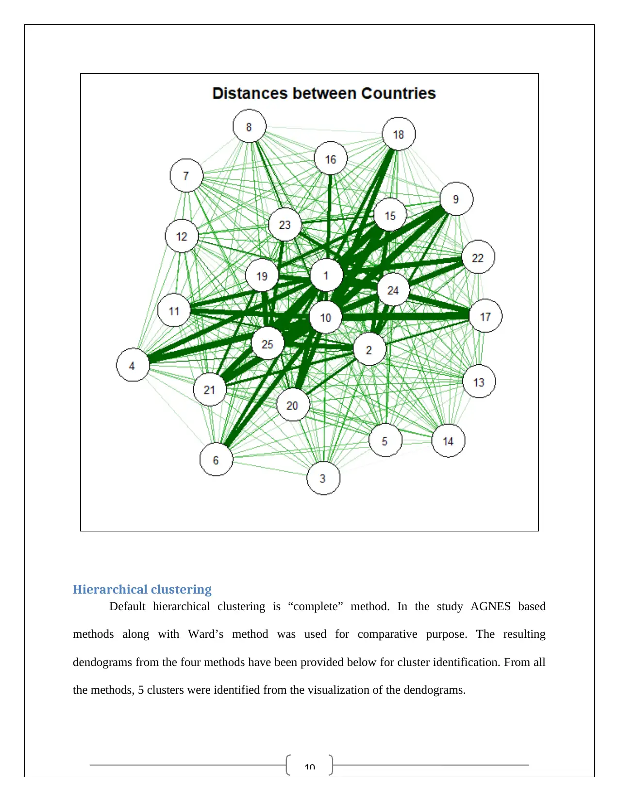
For the distance matrix data for Asian continent, Hierarchical clustering and Partition
clustering were performed to identify the zones of the location of the twenty five cities in the
dataset. The distance matrix was evaluated for exploratory purpose by the following heat map
and spring map. The red marked cells indicated the distances which pointed towards the
closeness of another country. The spring map was drawn to identify the proximity of two cities.
The bold line signified those counties which can isolated easily in a cluster. The dataset was
scaled by shifting the origin to median and changing the scale by absolute deviation from
median.
Question 2
Initial Data Discussion
For the distance matrix data for Asian continent, Hierarchical clustering and Partition
clustering were performed to identify the zones of the location of the twenty five cities in the
dataset. The distance matrix was evaluated for exploratory purpose by the following heat map
and spring map. The red marked cells indicated the distances which pointed towards the
closeness of another country. The spring map was drawn to identify the proximity of two cities.
The bold line signified those counties which can isolated easily in a cluster. The dataset was
scaled by shifting the origin to median and changing the scale by absolute deviation from
median.
10
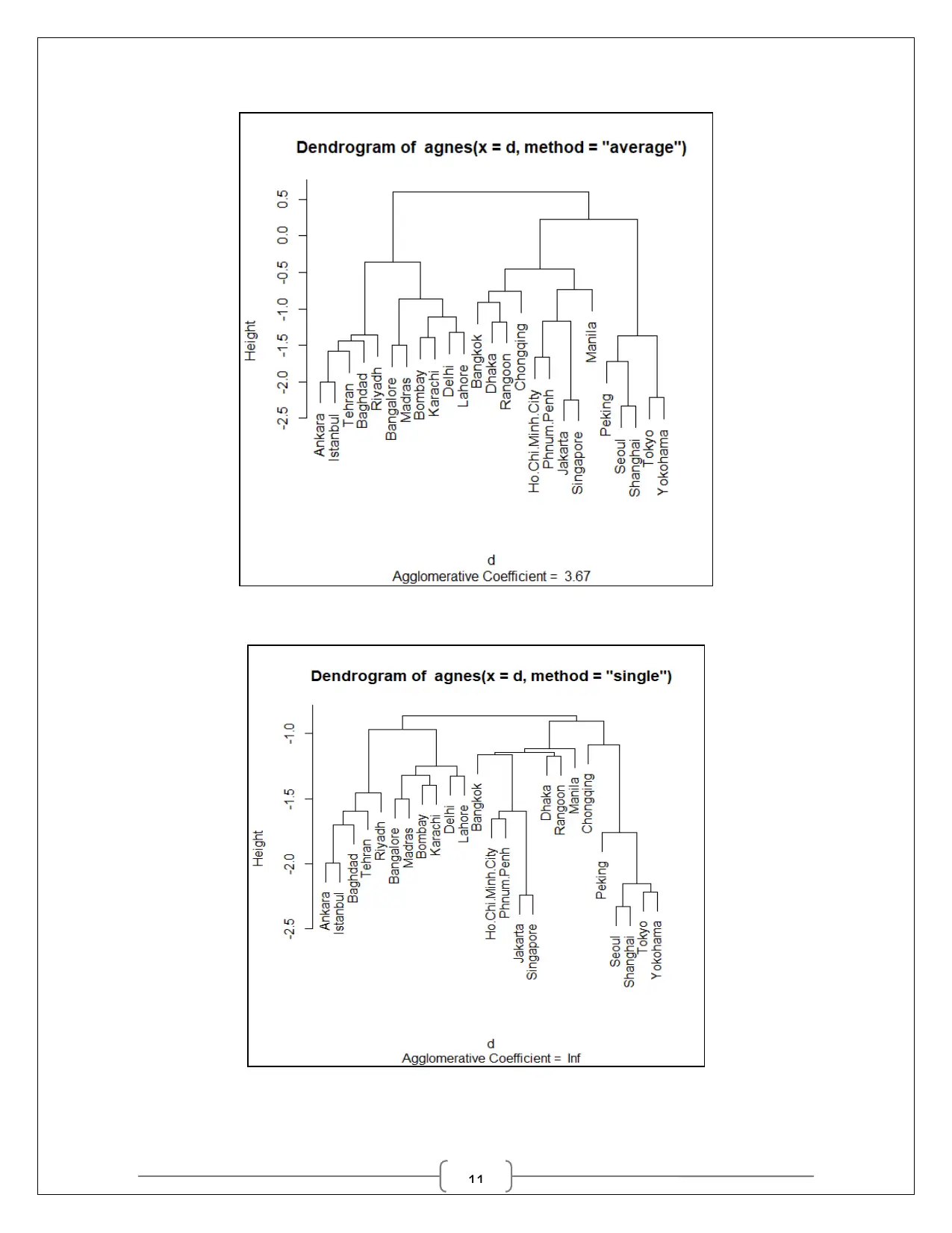
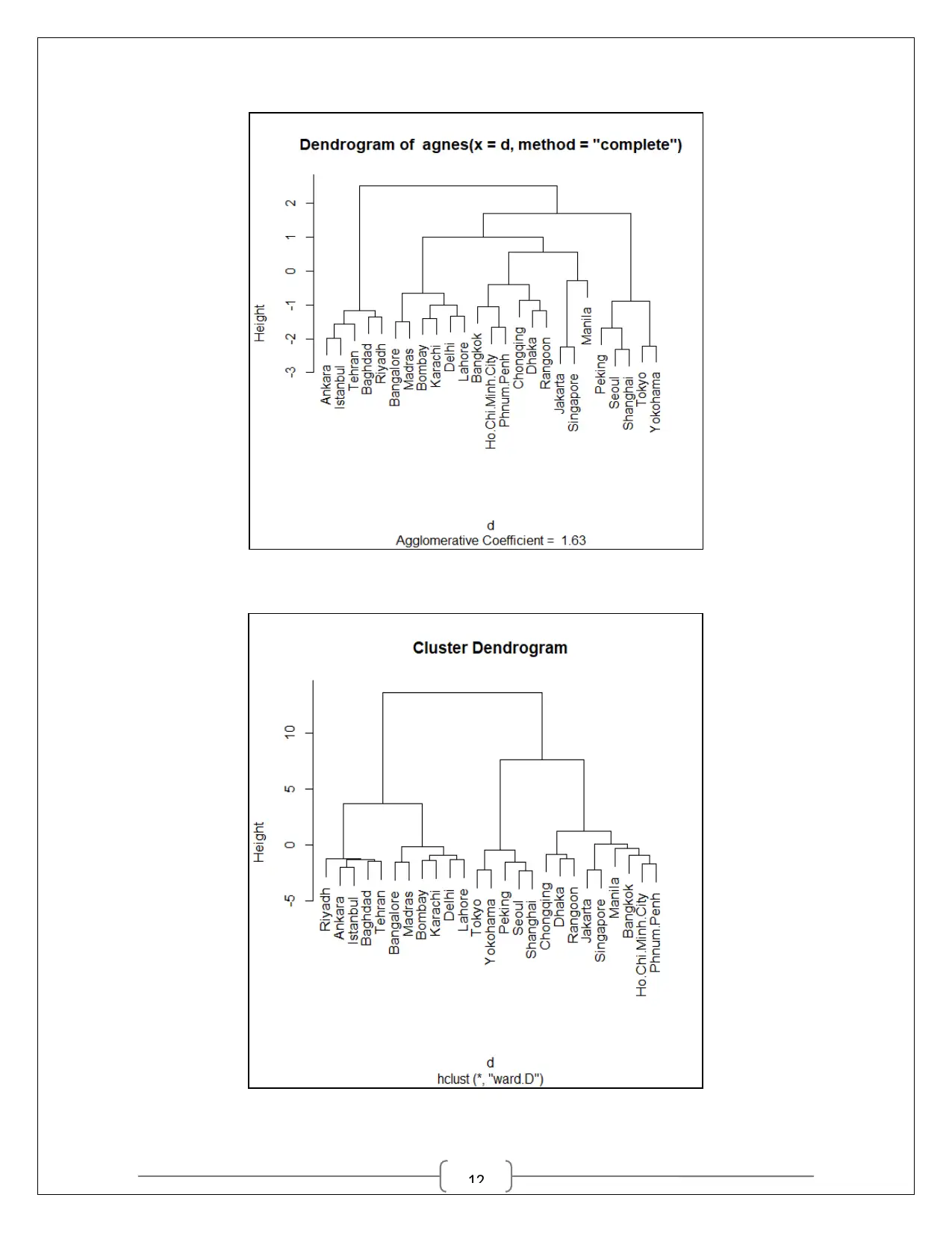
Hierarchical clustering
Default hierarchical clustering is “complete” method. In the study AGNES based
methods along with Ward’s method was used for comparative purpose. The resulting
dendograms from the four methods have been provided below for cluster identification. From all
the methods, 5 clusters were identified from the visualization of the dendograms.
Secure Best Marks with AI Grader
Need help grading? Try our AI Grader for instant feedback on your assignments.
11
12
13
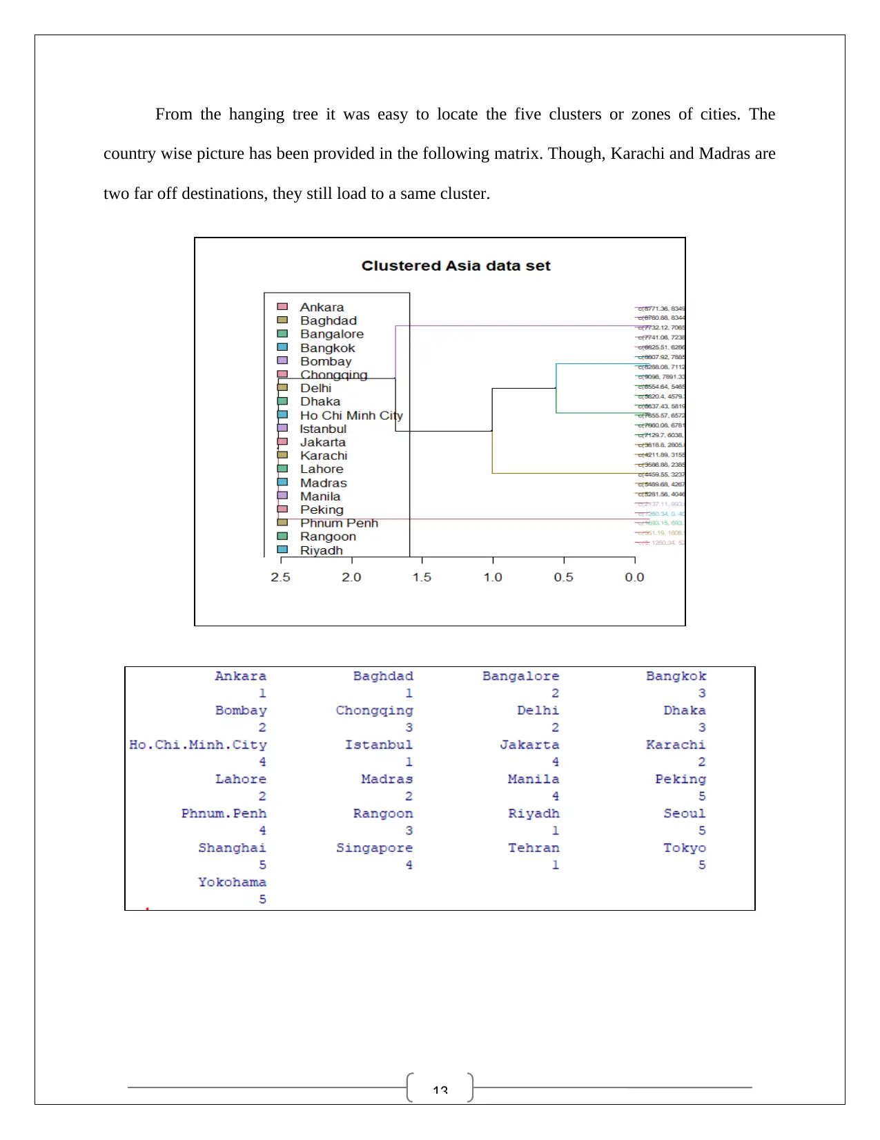
From the hanging tree it was easy to locate the five clusters or zones of cities. The
country wise picture has been provided in the following matrix. Though, Karachi and Madras are
two far off destinations, they still load to a same cluster.
From the hanging tree it was easy to locate the five clusters or zones of cities. The
country wise picture has been provided in the following matrix. Though, Karachi and Madras are
two far off destinations, they still load to a same cluster.
Paraphrase This Document
Need a fresh take? Get an instant paraphrase of this document with our AI Paraphraser
14
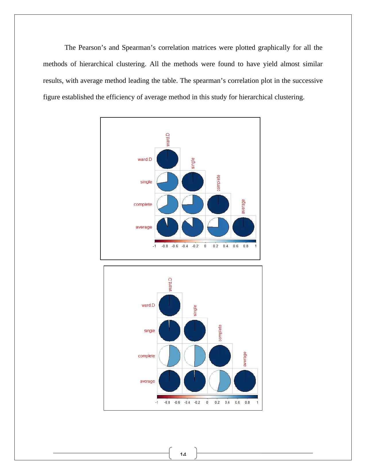
The Pearson’s and Spearman’s correlation matrices were plotted graphically for all the
methods of hierarchical clustering. All the methods were found to have yield almost similar
results, with average method leading the table. The spearman’s correlation plot in the successive
figure established the efficiency of average method in this study for hierarchical clustering.
15
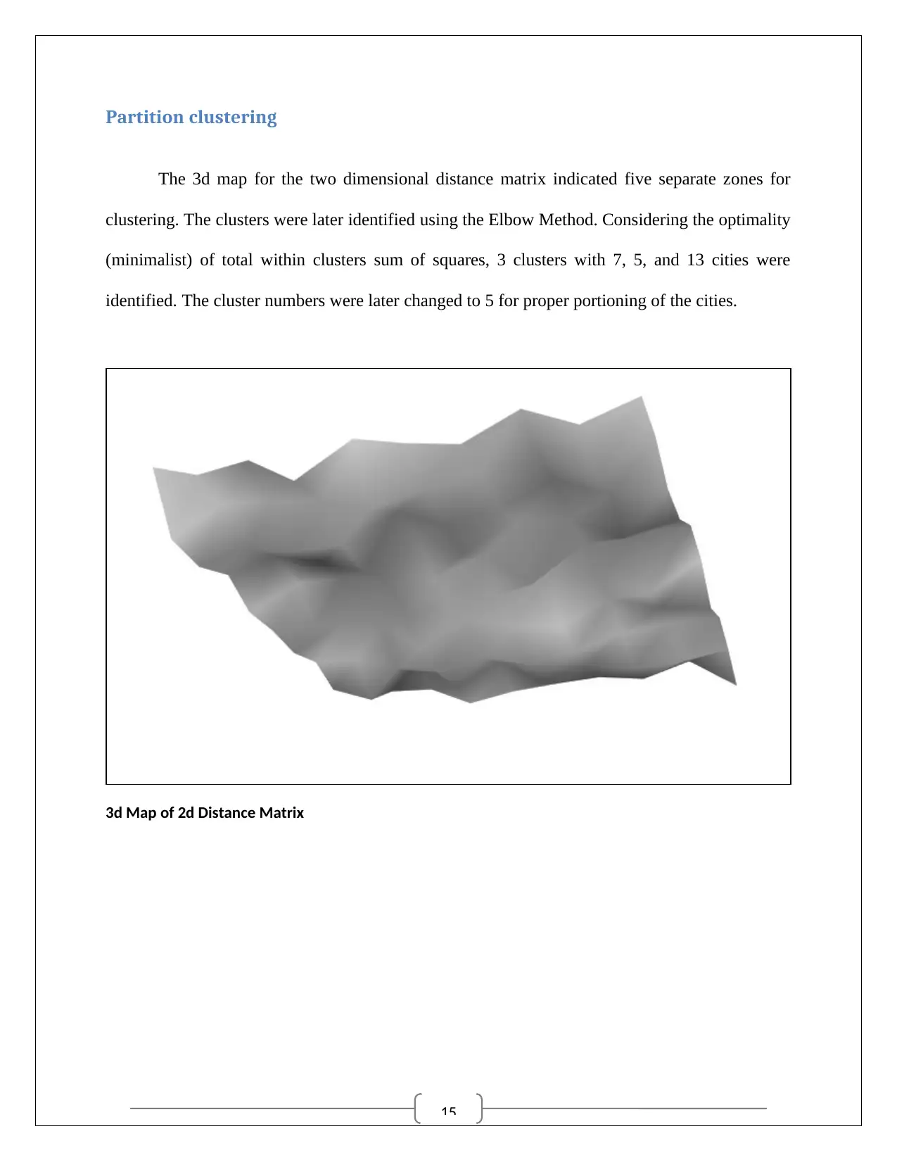
Partition clustering
The 3d map for the two dimensional distance matrix indicated five separate zones for
clustering. The clusters were later identified using the Elbow Method. Considering the optimality
(minimalist) of total within clusters sum of squares, 3 clusters with 7, 5, and 13 cities were
identified. The cluster numbers were later changed to 5 for proper portioning of the cities.
3d Map of 2d Distance Matrix
16
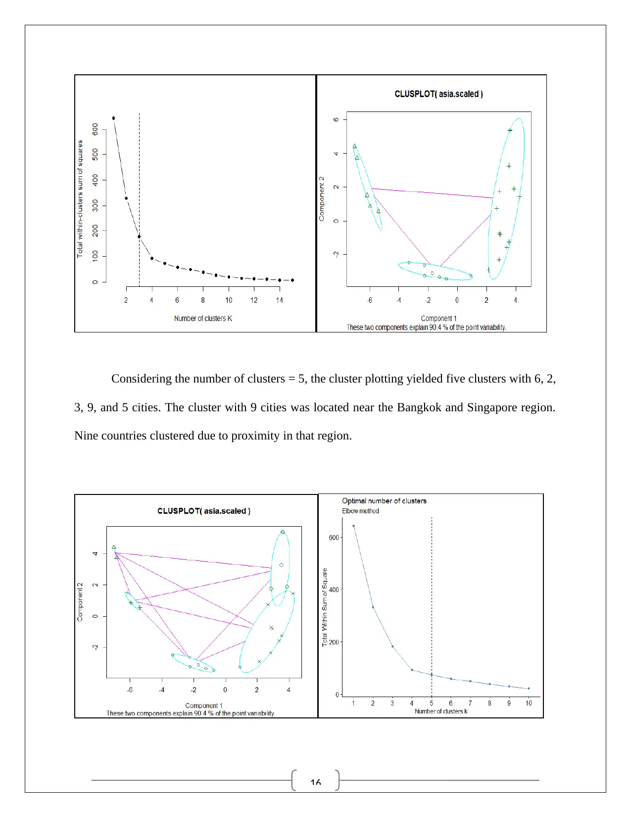
Considering the number of clusters = 5, the cluster plotting yielded five clusters with 6, 2,
3, 9, and 5 cities. The cluster with 9 cities was located near the Bangkok and Singapore region.
Nine countries clustered due to proximity in that region.
Considering the number of clusters = 5, the cluster plotting yielded five clusters with 6, 2,
3, 9, and 5 cities. The cluster with 9 cities was located near the Bangkok and Singapore region.
Nine countries clustered due to proximity in that region.
Secure Best Marks with AI Grader
Need help grading? Try our AI Grader for instant feedback on your assignments.
17
Discussion
The partitional clustering was based on choice of k-means or centers. Initial processing
suggested 3 clusters of cities with minimum total within clusters sum of squares at 75.4%. Later,
appropriate choice of clusters was decided on the basis of Elbow method, considering the
previous methods of cluster analysis. The 3d plot was an indicative figure in this case. Five zones
were identified, which were i) near Bangkok region, ii)near Delhi region, iii) near Yokahama
region, iv) near Bangalore region, and v) near Istanbul region.
Validation
No outlier distance was identified from the matrix, and proper choice of zones or clusters
of countries was identified to be 5. The initial clustering was able to reduce the SS of the total
clustering, but with formation of clusters with far-off countries. The solution with k=5 number of
partitioning was found to be appropriate from point of view of practical significance.
Conclusions
Both the hierarchical clustering and partitional clustering were efficient clustering
technique. But, considering the choice of clusters, hierarchical clustering was easy to interpret
because of the clear picture of the cluster loadings in dendograms. The k-means clustering had
the power of generating the optimal partitioning of the data points with minimum total within
clusters sum of squares.
In the present study, hierarchical clustering was efficient in deciding the number of
clusters compared to partitional clustering. In partitional clustering mutually exclusive spherical
shaped clusters were obtained. And in hierarchical clustering, based on agglomerative approach
and divisive approach, the countries were assumed as individual clusters and then clustered form
bottom to top direction in the tree (Yates et al., 2015).
18
References
Hanna, L. M. O., de Araújo, R. J. G., Vilarino, E. F. A., & Mayhew, A. S. B. (2016). The caries
experience and dentistry following evaluation of children submitted to antineoplastic
therapy. Journal of Research in Dentistry, 4(2), 45-50.
Yates, L. R., Gerstung, M., Knappskog, S., Desmedt, C., Gundem, G., Van Loo, P., ... & Li, Y.
(2015). Subclonal diversification of primary breast cancer revealed by multiregion
sequencing. Nature medicine, 21(7), 751.
1 out of 18
Your All-in-One AI-Powered Toolkit for Academic Success.
+13062052269
info@desklib.com
Available 24*7 on WhatsApp / Email
![[object Object]](/_next/static/media/star-bottom.7253800d.svg)
Unlock your academic potential
© 2024 | Zucol Services PVT LTD | All rights reserved.