Wage Analysis and Gender Inequality

This assignment analyzes the relationship between various factors and employee wages. It examines data on age, working hours, education level, number of children, and gender to understand how these variables influence earnings. The analysis also investigates the potential for gender inequality in wages, considering societal factors that might contribute to differences in pay between male and female employees.

Factors affecting wages of employed persons
Name:
Student Reg.:
School:
Department:
Course:
Task:
Lecturer:
Contents
Introduction..................................................................................................................................3

Research Problem........................................................................................................................3
Research hypothesis.....................................................................................................................3
Description of data.......................................................................................................................3
Data analysis methodology..........................................................................................................4
Results and discussion.................................................................................................................5
Descriptive statistics.................................................................................................................5
Inferential statistics...................................................................................................................6
Relationship between working hours and wage.......................................................................6
Relationship between gender and wages..................................................................................8
Conclusion...................................................................................................................................9
References....................................................................................................................................9

Introduction
Wages are affected by different factors from personal to group factors. When company or
organization is determining the salary and wages structure of employers, these factors should be
put into consideration labour unions, personal perception of wage, cost of living, government
legislation, ability to pay and demand and supply. At personal level factors that determine wages
include worker’s age and capacity, educational qualifications, worker experience, promotions
possibilities, gender and profit earned by the organization. Waged laborer’s can be divided into
employed which are self employment and waged employment and unemployment. Organization
perceives wages as hourly or salaried wages. Wages include relief pay, family allowance,
financial support and any other benefit originating from the firm.
Personal characteristics affect the wages level. Education qualification influences the wage one
get. According Lazear E. (2005) degree education result to higher pay than those employees who
have only college or high school qualification. The study established positive linear correlation
between wages and education. An increase in education qualification resulted to a higher pay and
vice versa.
In terms of age the older the employees the higher the experience and thus earn higher pay than
those who are younger. Old age is associated with experience and higher skills to do job better
compared to those who are young. Though higher age is associated with higher risk in term of
energy and more time consumed doing a job, (Kidd P., 1993).
Gender disparity also affects mechanism and passion of doing a task. Male are associated with
high vigor and mechanism and thus in jobs that require a lot of energy and mechanism tend to
get higher pay. Females attract more pay in jobs such as customer relation, marketing and front
office. These factors also affect male and female choices in employment, (Kunhn P. & Schuetze
H., 2001).
Research Problem
The study tries to answer the question of wages imbalance in different organization. What are the
factors that lead to this imbalance? Why are some employees doing the same job and in same
organization getting different wages?
Research hypothesis
 Number hours one spends working affect wages one get?
The report tries to identify if there exists any difference between employees working long hours
and those who are working in short hours.
 Gender affects wages of employee?
The study will try to identify how gender affects wages of employees.

Description of data
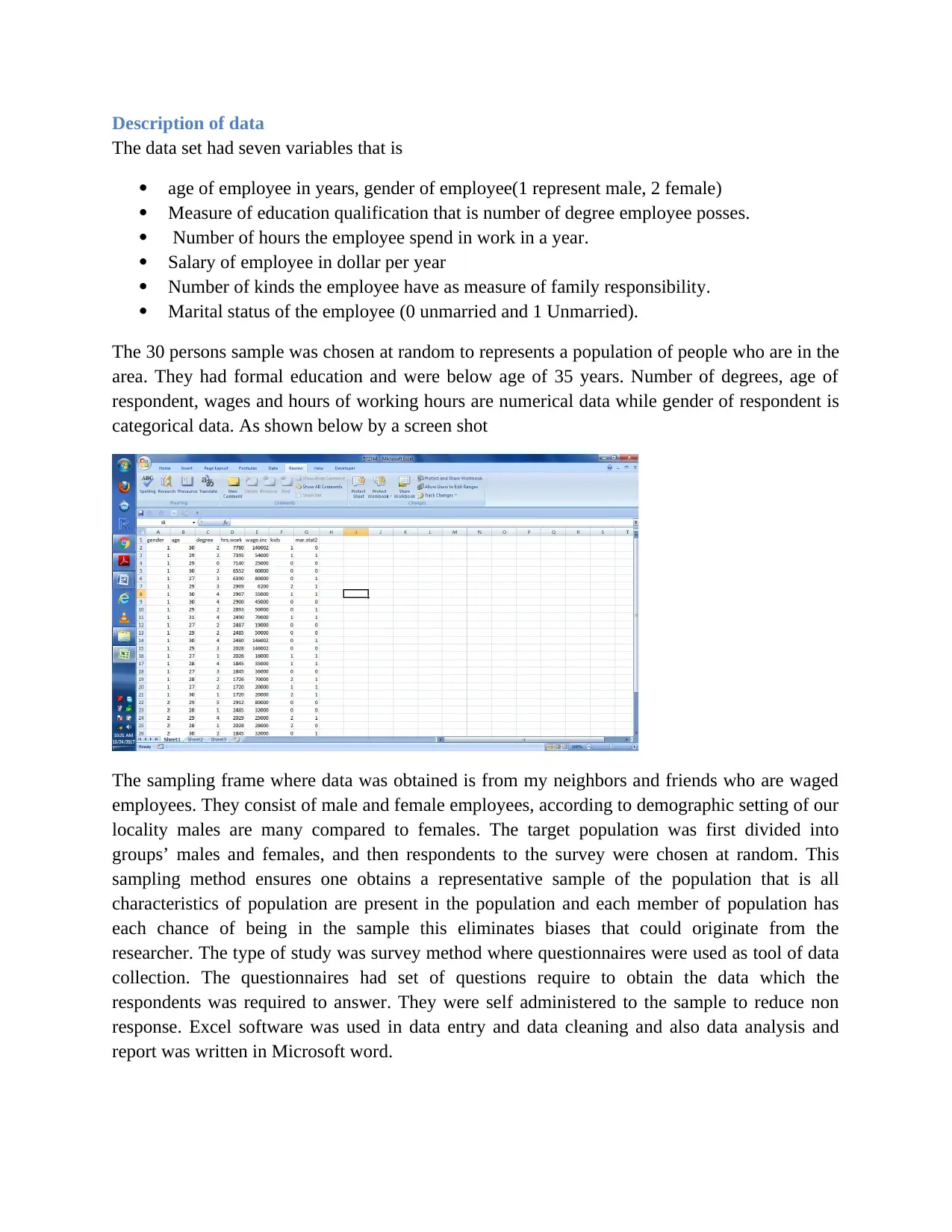
The data set had seven variables that is
 age of employee in years, gender of employee(1 represent male, 2 female)
 Measure of education qualification that is number of degree employee posses.
 Number of hours the employee spend in work in a year.
 Salary of employee in dollar per year
 Number of kinds the employee have as measure of family responsibility.
 Marital status of the employee (0 unmarried and 1 Unmarried).
The 30 persons sample was chosen at random to represents a population of people who are in the
area. They had formal education and were below age of 35 years. Number of degrees, age of
respondent, wages and hours of working hours are numerical data while gender of respondent is
categorical data. As shown below by a screen shot
The sampling frame where data was obtained is from my neighbors and friends who are waged
employees. They consist of male and female employees, according to demographic setting of our
locality males are many compared to females. The target population was first divided into
groups’ males and females, and then respondents to the survey were chosen at random. This
sampling method ensures one obtains a representative sample of the population that is all
characteristics of population are present in the population and each member of population has
each chance of being in the sample this eliminates biases that could originate from the
researcher. The type of study was survey method where questionnaires were used as tool of data
collection. The questionnaires had set of questions require to obtain the data which the
respondents was required to answer. They were self administered to the sample to reduce non
response. Excel software was used in data entry and data cleaning and also data analysis and
report was written in Microsoft word.

Data analysis methodology
Excel software was used as tool of analysis. The data analysis made use of inferential and
descriptive analysis method. Descriptive statistics are used to describe and summarized any data
set. They are used to describe what is in data or distribution of the data and provide a comparison
that can be used to compare set of data. When computing descriptive statistics one is at risk of
distorting the data. They include measure of location such as mean, median and mode and
measure of dispersion such as variance, range, quartile and deciles. In this study it explored
univariate variables. Inferential statistics infer and make conclusion on the population using
sample characteristics. They include regression analysis, hypothesis testing and confidence level
testing. The study utilized independent t-test is used to test significance, it checks if the mean of
two independent samples is significance different. Scatter diagram is a graphical method to
check linear relationship between two variables. When a linear relationship is identified
correlation analysis is used to check if the relationship is causal or not causal. The report will
cover the following histogram of number of hours worked and wages to check their distribution.
Scatter plot of working hours and gender to check any association or linear relationship between
the two variables. The relationship between wages and working hours is tested using regression
analysis. Regression analysis model which was utilized was y=a+bx where y is response
variable (wages) and x is predictor (working hours of employee per year).
Results and discussion
Descriptive statistics
To compute mean and variance the variable under study must be quantitative variables. The
average age of waged employee is 28.66 years. The standard deviation of age of employees 1.24,
this implies that majority of observed age lied near the mean. The average wage that the
employees earned in a year is 51200.87 dollars. The wage earned had an average working hours
of 2996.10 hours in year. This implies that earned on average 17.09 dollars per hour. The
average number of degree an employee has acquired is 2 and every employee has one child on
average. In order for one to earn 17.09 dollars per hour one must posse’s two degrees.
0
10000
20000
30000
40000
50000
60000
A histogram of number of hours work

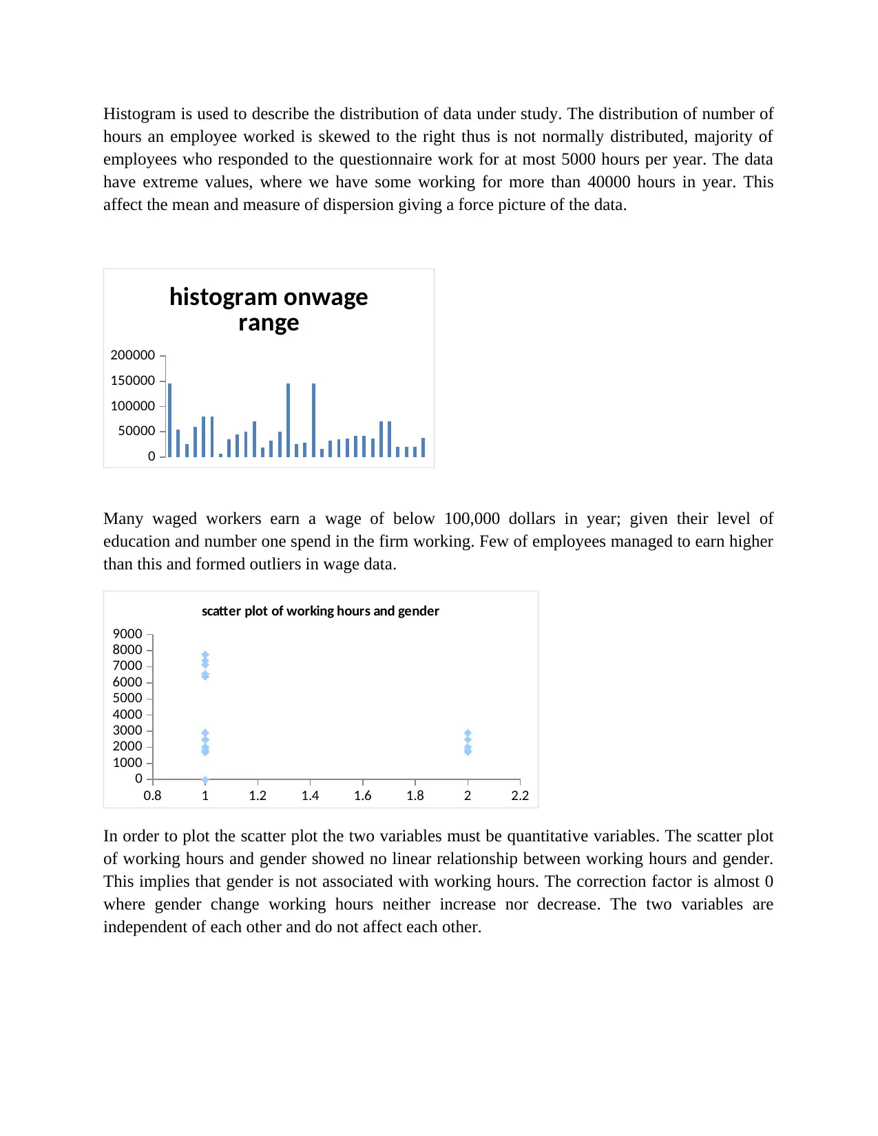
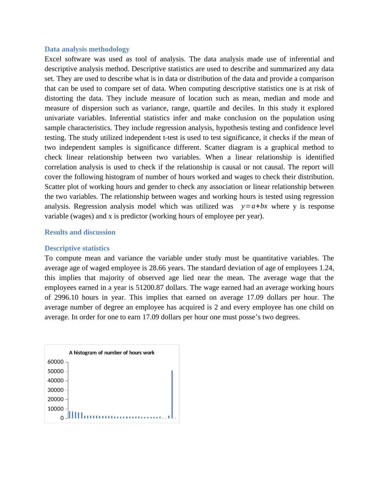
Histogram is used to describe the distribution of data under study. The distribution of number of
hours an employee worked is skewed to the right thus is not normally distributed, majority of
employees who responded to the questionnaire work for at most 5000 hours per year. The data
have extreme values, where we have some working for more than 40000 hours in year. This
affect the mean and measure of dispersion giving a force picture of the data.
Many waged workers earn a wage of below 100,000 dollars in year; given their level of
education and number one spend in the firm working. Few of employees managed to earn higher
than this and formed outliers in wage data.
0.8 1 1.2 1.4 1.6 1.8 2 2.2
0
1000
2000
3000
4000
5000
6000
7000
8000
9000
scatter plot of working hours and gender
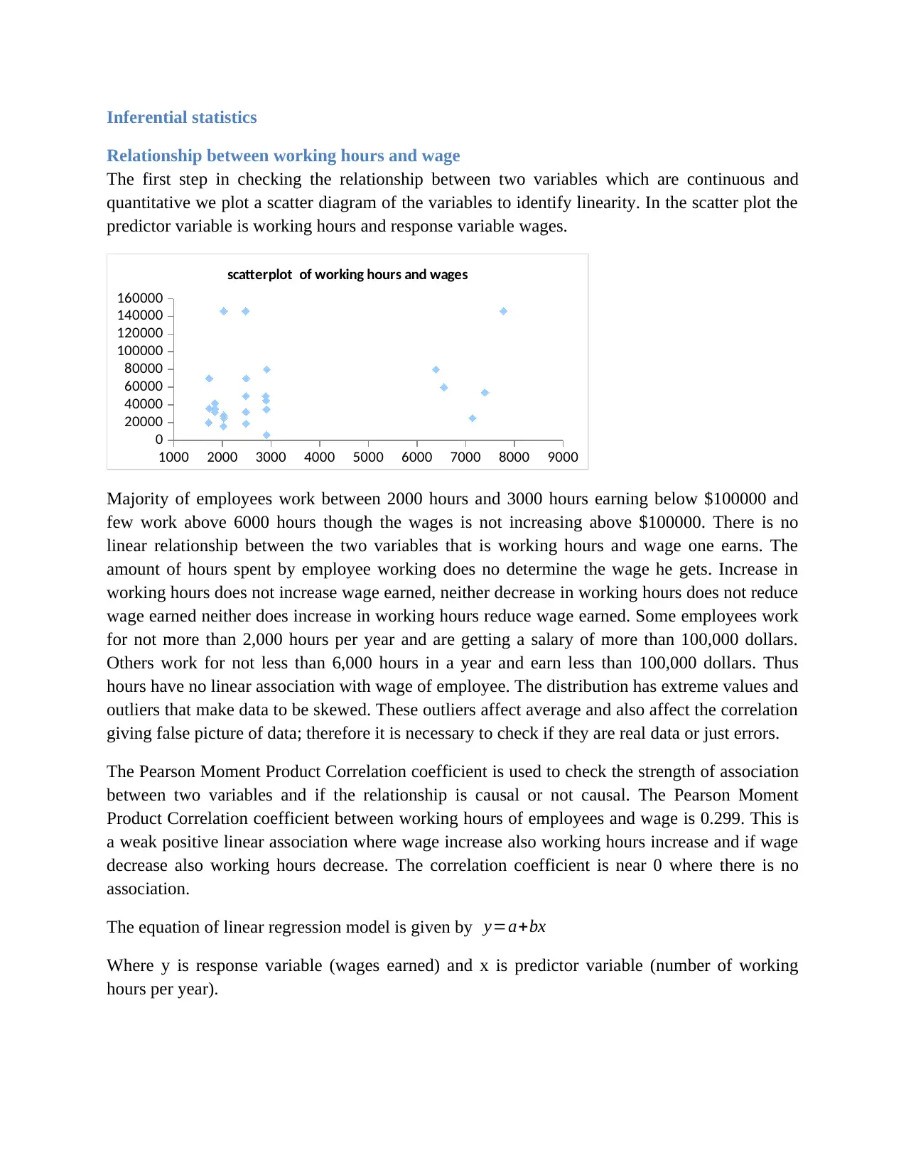
In order to plot the scatter plot the two variables must be quantitative variables. The scatter plot
of working hours and gender showed no linear relationship between working hours and gender.
This implies that gender is not associated with working hours. The correction factor is almost 0
where gender change working hours neither increase nor decrease. The two variables are
independent of each other and do not affect each other.
0
50000
100000
150000
200000
histogram onwage
range

Inferential statistics
Relationship between working hours and wage
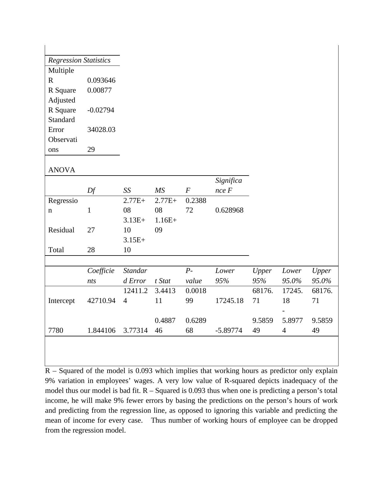
The first step in checking the relationship between two variables which are continuous and
quantitative we plot a scatter diagram of the variables to identify linearity. In the scatter plot the
predictor variable is working hours and response variable wages.
1000 2000 3000 4000 5000 6000 7000 8000 9000
0
20000
40000
60000
80000
100000
120000
140000
160000
scatterplot of working hours and wages
Majority of employees work between 2000 hours and 3000 hours earning below $100000 and
few work above 6000 hours though the wages is not increasing above $100000. There is no
linear relationship between the two variables that is working hours and wage one earns. The
amount of hours spent by employee working does no determine the wage he gets. Increase in
working hours does not increase wage earned, neither decrease in working hours does not reduce
wage earned neither does increase in working hours reduce wage earned. Some employees work
for not more than 2,000 hours per year and are getting a salary of more than 100,000 dollars.
Others work for not less than 6,000 hours in a year and earn less than 100,000 dollars. Thus
hours have no linear association with wage of employee. The distribution has extreme values and
outliers that make data to be skewed. These outliers affect average and also affect the correlation
giving false picture of data; therefore it is necessary to check if they are real data or just errors.
The Pearson Moment Product Correlation coefficient is used to check the strength of association
between two variables and if the relationship is causal or not causal. The Pearson Moment
Product Correlation coefficient between working hours of employees and wage is 0.299. This is
a weak positive linear association where wage increase also working hours increase and if wage
decrease also working hours decrease. The correlation coefficient is near 0 where there is no
association.
The equation of linear regression model is given by y=a+bx
Where y is response variable (wages earned) and x is predictor variable (number of working
hours per year).

SUMMARY
OUTPUT

Regression Statistics
Multiple
R 0.093646
R Square 0.00877
Adjusted
R Square -0.02794
Standard
Error 34028.03
Observati
ons 29
ANOVA
Df SS MS F
Significa
nce F
Regressio
n 1
2.77E+
08
2.77E+
08
0.2388
72 0.628968
Residual 27
3.13E+
10
1.16E+
09
Total 28
3.15E+
10
Coefficie
nts
Standar
d Error t Stat
P-
value
Lower
95%
Upper
95%
Lower
95.0%
Upper
95.0%
Intercept 42710.94
12411.2
4
3.4413
11
0.0018
99 17245.18
68176.
71
17245.
18
68176.
71
7780 1.844106 3.77314
0.4887
46
0.6289
68 -5.89774
9.5859
49
-
5.8977
4
9.5859
49
R – Squared of the model is 0.093 which implies that working hours as predictor only explain
9% variation in employees’ wages. A very low value of R-squared depicts inadequacy of the
model thus our model is bad fit. R – Squared is 0.093 thus when one is predicting a person’s total
income, he will make 9% fewer errors by basing the predictions on the person’s hours of work
and predicting from the regression line, as opposed to ignoring this variable and predicting the
mean of income for every case. Thus number of working hours of employee can be dropped
from the regression model.

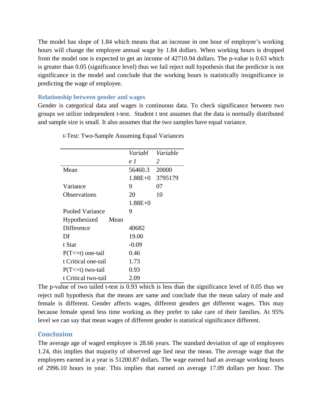
The model has slope of 1.84 which means that an increase in one hour of employee’s working
hours will change the employee annual wage by 1.84 dollars. When working hours is dropped
from the model one is expected to get an income of 42710.94 dollars. The p-value is 0.63 which
is greater than 0.05 (significance level) thus we fail reject null hypothesis that the predictor is not
significance in the model and conclude that the working hours is statistically insignificance in
predicting the wage of employee.
Relationship between gender and wages
Gender is categorical data and wages is continuous data. To check significance between two
groups we utilize independent t-test. Student t test assumes that the data is normally distributed
and sample size is small. It also assumes that the two samples have equal variance.
t-Test: Two-Sample Assuming Equal Variances
Variabl
e 1
Variable
2
Mean 56460.3 20000
Variance
1.88E+0
9
3795179
07
Observations 20 10
Pooled Variance
1.88E+0
9
Hypothesized Mean
Difference 40682
Df 19.00
t Stat -0.09
P(T<=t) one-tail 0.46
t Critical one-tail 1.73
P(T<=t) two-tail 0.93
t Critical two-tail 2.09
The p-value of two tailed t-test is 0.93 which is less than the significance level of 0.05 thus we
reject null hypothesis that the means are same and conclude that the mean salary of male and
female is different. Gender affects wages, different genders get different wages. This may
because female spend less time working as they prefer to take care of their families. At 95%
level we can say that mean wages of different gender is statistical significance different.
Conclusion
The average age of waged employee is 28.66 years. The standard deviation of age of employees
1.24, this implies that majority of observed age lied near the mean. The average wage that the
employees earned in a year is 51200.87 dollars. The wage earned had an average working hours
of 2996.10 hours in year. This implies that earned on average 17.09 dollars per hour. The

average number of degree an employee has acquired is 2 and every employee has one child on
average. In order for one to earn 17.09 dollars per hour one must posse’s two degrees. The
Pearson Moment Product Correlation coefficient between working hours of employees and wage
is 0.299. This is a weak positive linear association where wage increase also working hours
increase and if wage decrease also working hours decrease. The correlation coefficient is near 0
where there is no association. The model of predicting wages using working hours of employee
was a bad fit. Working hours can not be used to predict wages and we dropped it from the model
and conclude that wages is affected by other factors other than working hour of the employee.
Gender affects wages, different genders get different wages. This may because female spend less
time working as they prefer to take care of their families. The mean salaries of female are
different from that of male.