Factors influencing the Import Expenditure

Running Header: Factors influencing the import expenditure 1
Factors influencing the import expenditure
Students name:
ID:
Institution:

Factors influencing the import expenditure 2
Introduction
The study examines the relationship between import expenditure (IMPORTS), Consumer
Price Index (CPI) and GDP in the UK from 1985 to 2015. The study examines the import
function while evaluating the significance of the variables (CPI and GDP) which influences
the import expenditure. Simple linear regression models were used in investigating the
relationship between import expenditure and CPI and GDP separately while a multiple
regression analysis was used in investigating the relationship between import expenditure and
CPI and GDP together.
Part (A): Simple Linear Regression Model
Assumptions of Classical Linear Regression Model (CLRM)
According to Hose & Hans (2019), there are seven assumptions of CLRM.
First Assumption: The parameters of a regression model are. Violating this assumption
produces errors during extrapolation of the assumed model.
Second Assumption: The regressors are not stochastic or fixed. Violating this assumption
produces unreasonable predictions especially beyond the range of sample data.
Third Assumption: The mean value of the error term is 0 given the values of the independent
variables. Violation of this assumption biases the regression coefficient produced by the OLS.
Forth Assumption: Each error term variance given the independent variables values is
homoscedastic. Violating this assumption leads to the regression coefficient produced to be
less reliable since the data point across each independent variable does not influence equally.
Fifth Assumption: The error terms belonging to two different observations have no
correlation.
Sixth Assumption: The independent variables have no perfect linear relationship. Hence there
is no multicollinearity. Violating assumptions 5 and 6 causes the regression coefficient
variance to increase.

Factors influencing the import expenditure 3
Assumption 7: Correct specification of the regression model in use. Hence, there is no bias or
specific error. Violating this assumption makes the regression coefficient to be less reliable.
Properties of OLS Estimators
The linear property of the OLS estimators suggest than the OLS belongs in an estimator class
which is linear to the dependent variable (Rahman et al,, 2018). The estimator needs to be an
unbiased estimator of the true population or parameter values making it the most desirable
property of any estimator. The best minimum variance property places an estimator as being
efficient. Thus, the estimator will have the variance that is the least when taking all unbiased
estimators of the unknown population parameter. The asymptotic unbiasedness means when
the sample size of an OLS estimator increases, the unbiasedness disappears. Finally, an
estimator is pointed out to be coherent if its value approached the true parameter population
value when there is an increase in the sample size.
Scatterplots
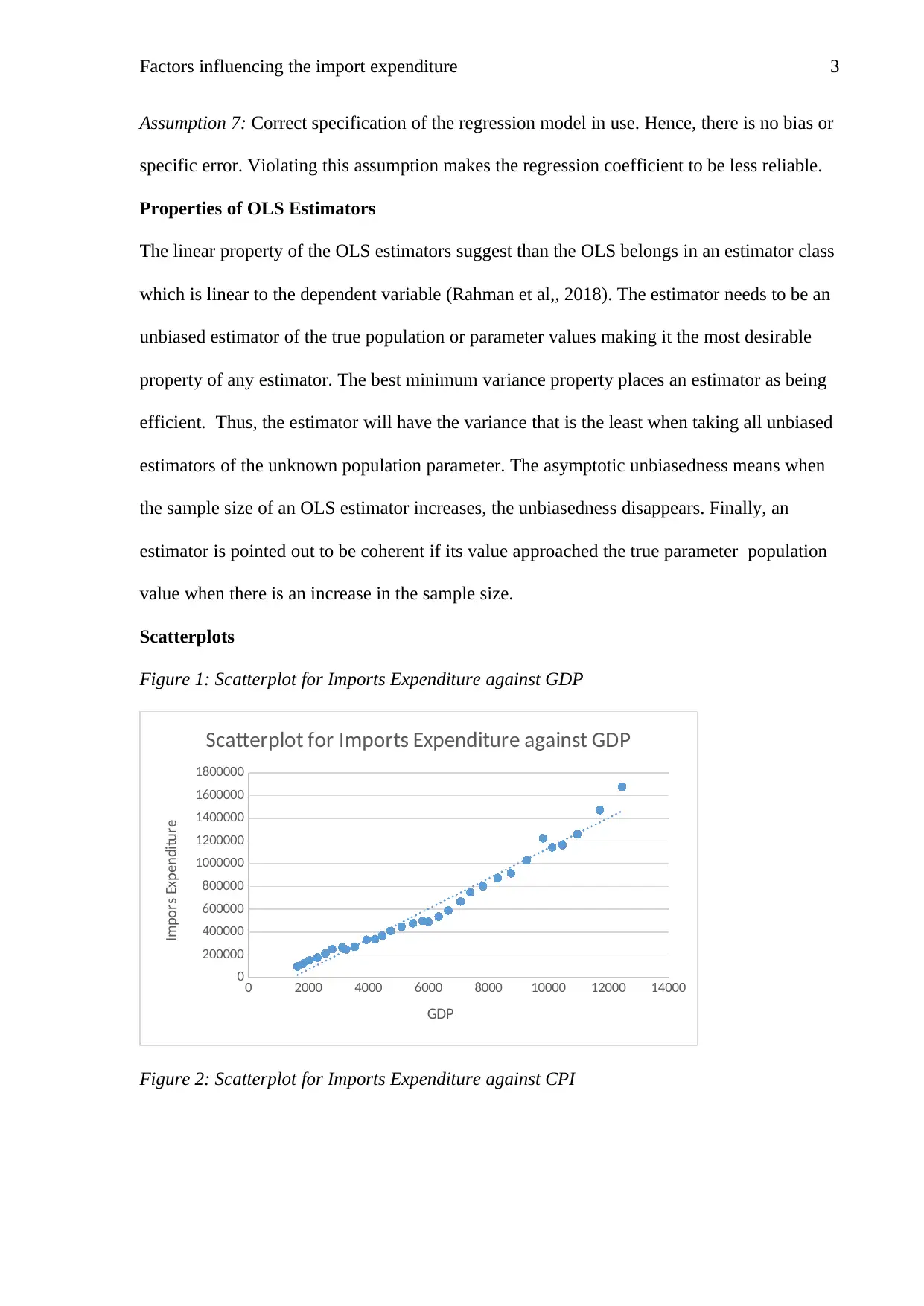
Figure 1: Scatterplot for Imports Expenditure against GDP
0 2000 4000 6000 8000 10000 12000 14000
0
200000
400000
600000
800000
1000000
1200000
1400000
1600000
1800000
Scatterplot for Imports Expenditure against GDP
GDP
Impors Expenditure
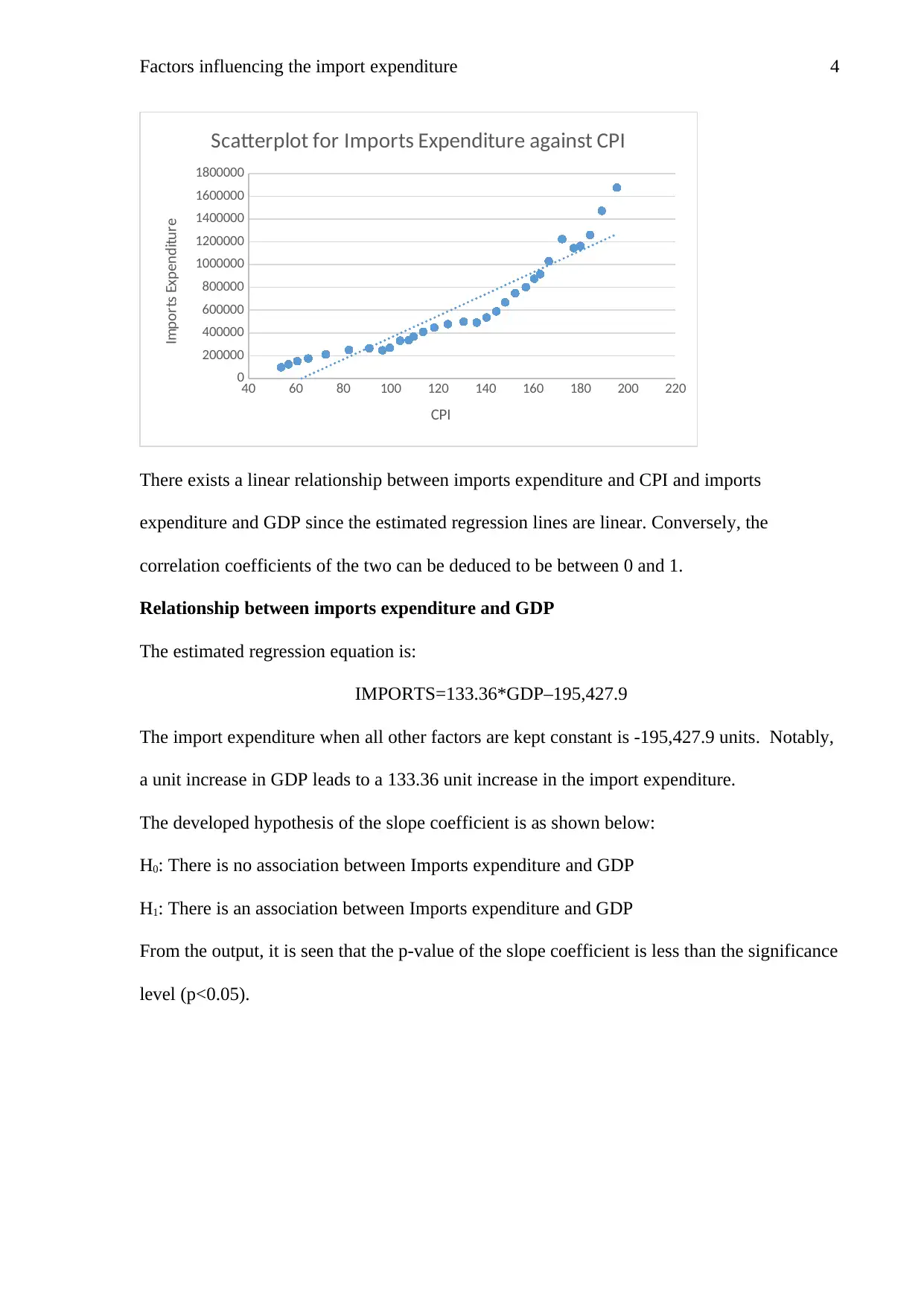
Figure 2: Scatterplot for Imports Expenditure against CPI

Factors influencing the import expenditure 4
40 60 80 100 120 140 160 180 200 220
0
200000
400000
600000
800000
1000000
1200000
1400000
1600000
1800000
Scatterplot for Imports Expenditure against CPI
CPI
Imports Expenditure
There exists a linear relationship between imports expenditure and CPI and imports
expenditure and GDP since the estimated regression lines are linear. Conversely, the
correlation coefficients of the two can be deduced to be between 0 and 1.
Relationship between imports expenditure and GDP
The estimated regression equation is:
IMPORTS=133.36*GDP–195,427.9
The import expenditure when all other factors are kept constant is -195,427.9 units. Notably,
a unit increase in GDP leads to a 133.36 unit increase in the import expenditure.
The developed hypothesis of the slope coefficient is as shown below:
H0: There is no association between Imports expenditure and GDP
H1: There is an association between Imports expenditure and GDP
From the output, it is seen that the p-value of the slope coefficient is less than the significance
level (p<0.05).

Factors influencing the import expenditure 5
Since the p-value lies in the rejection region, we choose to reject the null hypothesis. Hence,
there is a statistically significant relationship between imports expenditure and GDP.
Coefficient of Determination
The R2 is 0.97. Hence, 97% of the variability in the model is accounted for by factors within
the model while 3% is accounted for by factors not within the model.
The hypotheses developed for the F-test for the explanatory power of the model are:
H0: Model with no independent variables fits the data together with the model
H1: The model with an independent variable fits the data better than the model with an
intercept only
The value of the F-statistic was 933.69, as shown in the output summary table. Consequently,
the p-value of the f-statistic was 0.00.
Since p<0.05, we choose to reject the null hypothesis. Hence, the model with an independent
variable fits the data better than the model with an intercept only.

Factors influencing the import expenditure 6
Relationship between imports expenditure and CPI
The estimated regression equation is:
IMPORTS=9,545.7*CPI–595,264
The import expenditure when all other factors are kept constant is -595,264 units. Moreover,
a unit increase in CPI leads to a 9,545.7 unit increase in the import expenditure.
The developed hypothesis of the slope coefficient statistical significance is as shown below:
H0: IMPORTS = CPI
H1: IMPORTS ≠ CPI
The p-value of the slope coefficient is less than the significance level (p<0.05).
Since the p-value lies in the rejection region, we choose to reject the null hypothesis. Hence,
there is a relationship between imports expenditure and CPI.
Coefficient of Determination
The R2 is 0.88. Hence, 88% of the variability in the model is accounted for by factors within
the model while 12% is accounted by factors which are not within the model.
The hypotheses developed for the F-test for the explanatory power of the model are:
H0: Model with no independent variables fits the data together with the model
H1: The model with an independent variable fits the data better than the model with an
intercept only
The value of the F-statistic and its p-value were 209.94 and 0.00 respectively.

Factors influencing the import expenditure 7
Since p<0.05, we choose to reject the null hypothesis. Hence, model with an independent
variable fits the data better than the model with an intercept only.
Predicted Import Expenditure
Sample regression equation (1) is as shown:
IMPORTS=133.36*GDP–195,427.9
The predicted import expenditure for years 2010, 2011 and 2012 are as shown in the table
below.
Table 1: Imports prediction from model
Unlike the actual imports expenditure, the predicted imports expenditure is seen to be
increasing linearly whereas the actual imports fluctuated within the three years. Hence, the
predicted model is linear in nature and does not consider uncertainties in the market.
Regression through function forms
The slope coefficients in both simple linear regressions mean that the two variables are a
function of the dependent variable as both models have shown that they are positive. Hence,
they are meaningful in the context of import expenditure and CPI and GDP.
Different function forms were adopted by taking the natural logarithm of all variables.
LNIMPORTS=2+1.29*LNGDP

Factors influencing the import expenditure 8
A one percent increase in the GDP would yield a 1.29% increase in the imports expenditure.
LNIMPORTS=3.6+1.99*LNCPI
Similarly, a one percent increase in the CPI would yield a 3.6% increase in the imports
expenditure.
It can be concluded that there is an elastic relationship between Imports and GDP and CPI.
Hypothesis testing using log-transformed variables
The developed hypothesis of the slope coefficient statistical significance is as shown below:
Hypothesis 1
H0: LNIMPORTS = LNCPI
H1: LNIMPORTS ≠ LNCPI
Hypothesis 2
H0: LNIMPORTS = LNGDP
H1: LNIMPORTS ≠ LNGDP
The p-value of the slope coefficients were less than the significance level (p<0.05). Hence, we
choose to reject the null hypothesis. Thus:
a. There is a statistically significant relationship between LNIMPORTS and LNCPI.
b. There is a statistically significant relationship between LNIMPORTS and LNGDP
Generally, it is observed that the results of the answers, hypothesis and final conclusion do not
differ from the previous variables which were yet to be transformed.
Test for explanatory power through F-test
The R2 between LNIMPORTS and LNCPI is 0.96. Hence, 96% of the variability in the model
is accounted for by factors within the model while 4% is accounted for by factors which are
not within the model.

Factors influencing the import expenditure 9
Conversely, the R2 between LNIMPORTS and LNGDP is 0.989. Thus, 98.9% of the
variability in the model is accounted by factors within the model while 1.1% is accounted by
factors which are not within the model.
The hypotheses developed for the two F-test for the explanatory power of the model are:
H0: Model with no independent variables fits the data together with the model
H1: The model with an independent variable fits the data better than the model with an
intercept only
The values of the F-statistic and the p-value were 750.46 and 0.00; and 2686.48 and 0.00
respectively. Since p<0.05, we choose to reject the null hypothesis. Hence, the model with an
independent variable fits the data better than the model with an intercept only.
Appropriate functional form
The regression functional form with the log-transformed variable is better and more
appropriate. The R2 of the two simple linear regression increased once the variables were
transformed. Thus, the regression was able to contain majority of the variability while the
instances of variabilities being explained by factors not within the model being minimised.
Part (B): Multiple Regression Analysis
Multiple Regression using the log-transformed variables
LNIMPORTS=1.41+1.85*LNGDP+0.87*LNCPI
All factors kept constant, a 1% increase in the GDP would yield a 1.85% increase in the
imports expenditure. However, keeping all factors constant, a 1% increase in the CPI yields a
0.87% decrease in the imports expenditure.
Comparing LNGDP in simple linear regression and multiple regression
The R2 of LNGDP are not different since they both have a positive influence on the log
transformed Imports expenditure. Consequently, the two coefficients remain to be statistically
significant influencers of LNGDP.

Factors influencing the import expenditure 10
The R2 from the multiple regression model is 0.992. Hence 99.2% of the variability is
explained by factors within the model while 0.8% is explained by factors not within the
model.
The R2 from the estimated linear regression of LNIMPORTS on LNGDP is 0.989 while the
one calculated in the multiple regression is 0.992. The multiple regression with the
transformed variable is the most appropriate since its R2 is greater than the coefficient of
determination of LNIMPORTS on LNGDP.
Significance of correlation coefficients
The developed hypothesis of the slope coefficient of LNGDP is as shown below:
H0: β2=0
H1: β2≠0
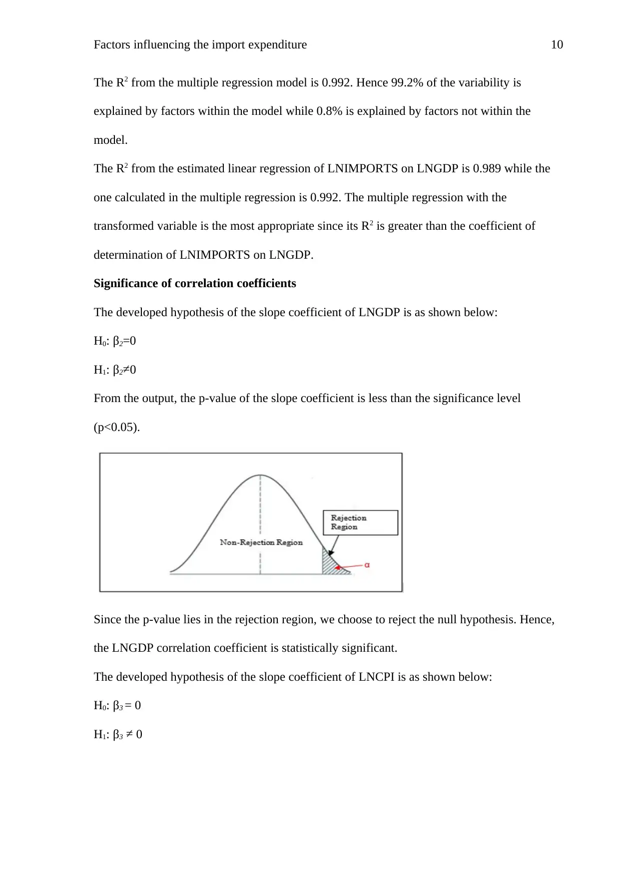
From the output, the p-value of the slope coefficient is less than the significance level
(p<0.05).
Since the p-value lies in the rejection region, we choose to reject the null hypothesis. Hence,
the LNGDP correlation coefficient is statistically significant.
The developed hypothesis of the slope coefficient of LNCPI is as shown below:
H0: β3 = 0
H1: β3 ≠ 0

Factors influencing the import expenditure 11
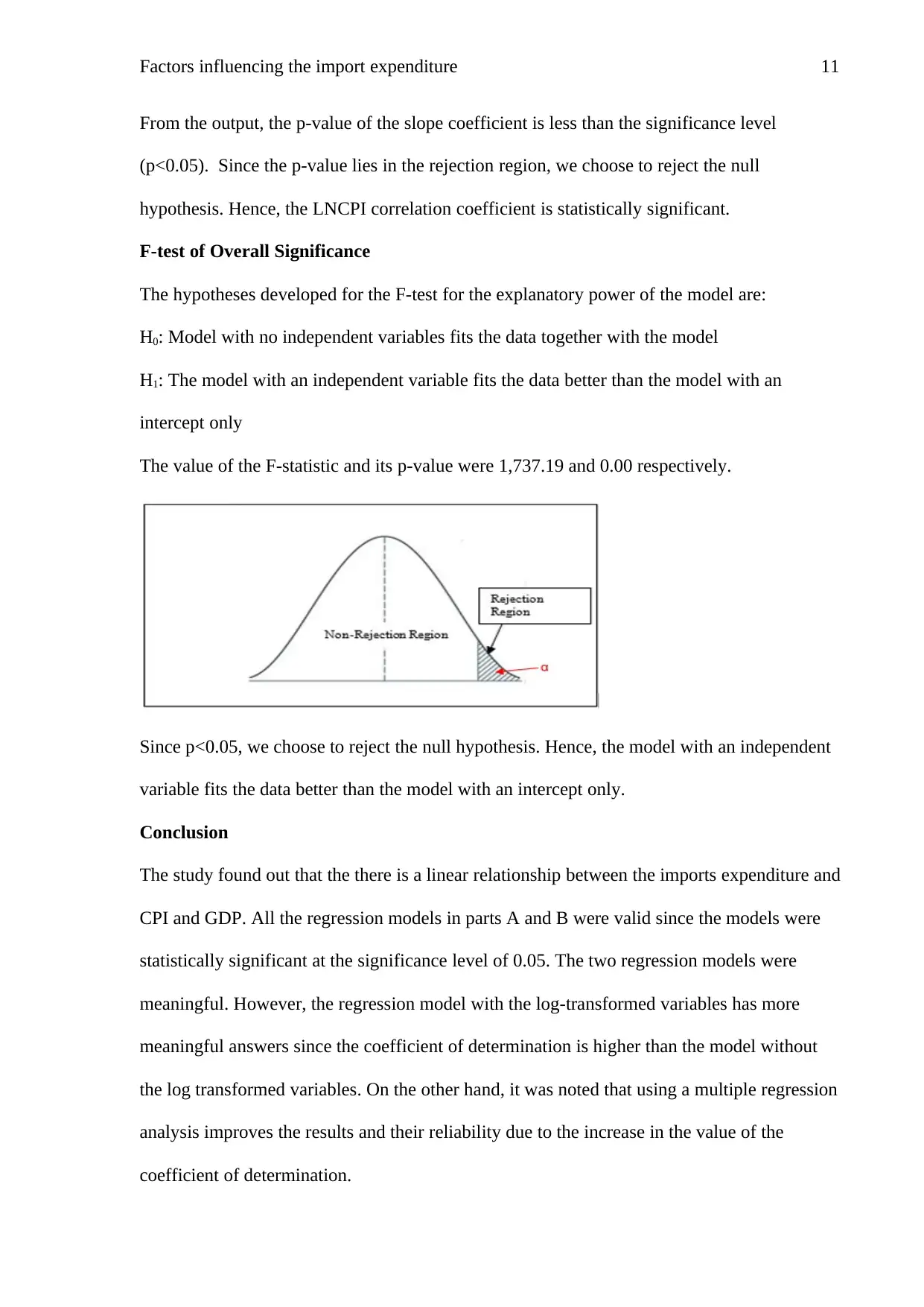
From the output, the p-value of the slope coefficient is less than the significance level
(p<0.05). Since the p-value lies in the rejection region, we choose to reject the null
hypothesis. Hence, the LNCPI correlation coefficient is statistically significant.
F-test of Overall Significance
The hypotheses developed for the F-test for the explanatory power of the model are:
H0: Model with no independent variables fits the data together with the model
H1: The model with an independent variable fits the data better than the model with an
intercept only
The value of the F-statistic and its p-value were 1,737.19 and 0.00 respectively.
Since p<0.05, we choose to reject the null hypothesis. Hence, the model with an independent
variable fits the data better than the model with an intercept only.
Conclusion
The study found out that the there is a linear relationship between the imports expenditure and
CPI and GDP. All the regression models in parts A and B were valid since the models were
statistically significant at the significance level of 0.05. The two regression models were
meaningful. However, the regression model with the log-transformed variables has more
meaningful answers since the coefficient of determination is higher than the model without
the log transformed variables. On the other hand, it was noted that using a multiple regression
analysis improves the results and their reliability due to the increase in the value of the
coefficient of determination.

Factors influencing the import expenditure 12
Reference
Hose, D. and Hanss, M., 2019. Fuzzy linear least squares for the identification of possibilistic
regression models. Fuzzy Sets and Systems, 367, pp.82-95.
Rahman, M.N., Das, S., Yadav, I., Kumar, P., Sophia, S.F., Gayathri, J., Mirabi, V.R.,
Ardestani, A.S., Pirbasti, M.F., Rao, P.H. and Arora, H., 2018. Macroeconomic
variables of India and finite sample properties of OLS under classical
assumptions. Pacific Business Review International, 10(8), pp.7-14.

Factors influencing the import expenditure 13
Appendix
Table 1: Relationship between IMPORTS and GDP
Table 2: Relationship between IMPORTS and CPI
Table 3: Relationship between LNIMPORTS and LNGDP

Factors influencing the import expenditure 14
Table 4: Relationship between LNIMPORTS and LNCPI
Table 5: Relationship between LNIMPORTS and LNGDP and LNCPI

Factors influencing the import expenditure 15