THE FINAL INDIVIDUAL ACTIVITY

Running Head: FINAL INDIVIDUAL ACTIVITY 1
Final Individual Activity
Student’s Name
Institutional Affiliation

FINAL INDIVIDUAL ACTIVITY 2
Final Individual Activity
Discussion In the research process for Frito-Lay Company, many different numerical questions
were raised regarding Frito-Lay products, advertising techniques, and purchase patterns among
Hispanics. In each of these areas, statistics—in particular, hypothesis testing—plays a central
role. Using the case information and the concepts of statistical hypothesis testing, discuss the
following:
1. 1 Many proportions were generated in the focus groups and market research that were
conducted for this project, including the proportion of the market that is Hispanic, the
proportion of Hispanic grocery shoppers that are women, the proportion of chip purchasers that
are teens, and so on. Use techniques you learned to analyze each of the following and discuss
how the results might affect marketing decision makers regarding the Hispanic market.
a.The case information stated that 63% of all U.S. Hispanics are Mexican American. How might
we test that figure? Suppose 850 U.S. Hispanics are randomly selected using U.S. Census
Bureau information. Suppose 575 state that they are Mexican Americans. Test the 63%
percentage using an alpha of .05.
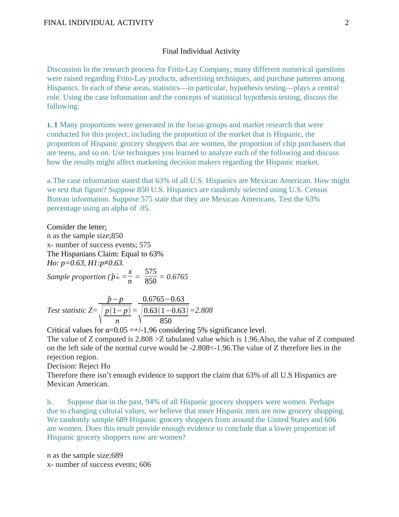
Consider the letter;
n as the sample size;850
x- number of success events; 575
The Hispanians Claim: Equal to 63%
Ho: p=0.63, H1:p≠0.63.
Sample proportion ( ^p ¿ = x
n = 575
850 = 0.6765
Test statistic Z=
^p− p
√ p(1− p)
n
=
0.6765−0.63
√ 0.63(1−0.63)
850
=2.808
Critical values for α=0.05 =+/-1.96 considering 5% significance level.
The value of Z computed is 2.808 >Z tabulated value which is 1.96.Also, the value of Z computed
on the left side of the normal curve would be -2.808<-1.96.The value of Z therefore lies in the
rejection region.
Decision: Reject Ho
Therefore there isn’t enough evidence to support the claim that 63% of all U.S Hispanics are
Mexican American.
b. Suppose that in the past, 94% of all Hispanic grocery shoppers were women. Perhaps
due to changing cultural values, we believe that more Hispanic men are now grocery shopping.
We randomly sample 689 Hispanic grocery shoppers from around the United States and 606
are women. Does this result provide enough evidence to conclude that a lower proportion of
Hispanic grocery shoppers now are women?
n as the sample size;689
x- number of success events; 606

FINAL INDIVIDUAL ACTIVITY 3
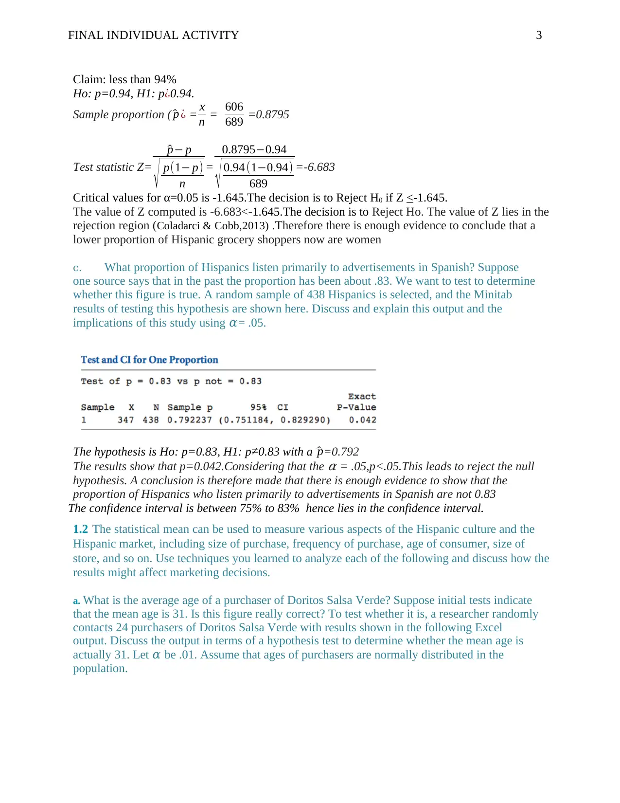
Claim: less than 94%
Ho: p=0.94, H1: p¿0.94.
Sample proportion ( ^p ¿ = x
n = 606
689 =0.8795
Test statistic Z=
^p− p
√ p(1− p)
n
=
0.8795−0.94
√ 0.94 (1−0.94)
689
=-6.683
Critical values for α=0.05 is -1.645.The decision is to Reject H0 if Z <-1.645.
The value of Z computed is -6.683<-1.645.The decision is to Reject Ho. The value of Z lies in the
rejection region (Coladarci & Cobb,2013) .Therefore there is enough evidence to conclude that a
lower proportion of Hispanic grocery shoppers now are women
c. What proportion of Hispanics listen primarily to advertisements in Spanish? Suppose
one source says that in the past the proportion has been about .83. We want to test to determine
whether this figure is true. A random sample of 438 Hispanics is selected, and the Minitab
results of testing this hypothesis are shown here. Discuss and explain this output and the
implications of this study using 𝛼= .05.
The hypothesis is Ho: p=0.83, H1: p≠0.83 with a ^p=0.792
The results show that p=0.042.Considering that the
𝛼 = .05,p<.05.This leads to reject the null
hypothesis. A conclusion is therefore made that there is enough evidence to show that the
proportion of Hispanics who listen primarily to advertisements in Spanish are not 0.83
The confidence interval is between 75% to 83% hence lies in the confidence interval.
1.2 The statistical mean can be used to measure various aspects of the Hispanic culture and the
Hispanic market, including size of purchase, frequency of purchase, age of consumer, size of
store, and so on. Use techniques you learned to analyze each of the following and discuss how the
results might affect marketing decisions.
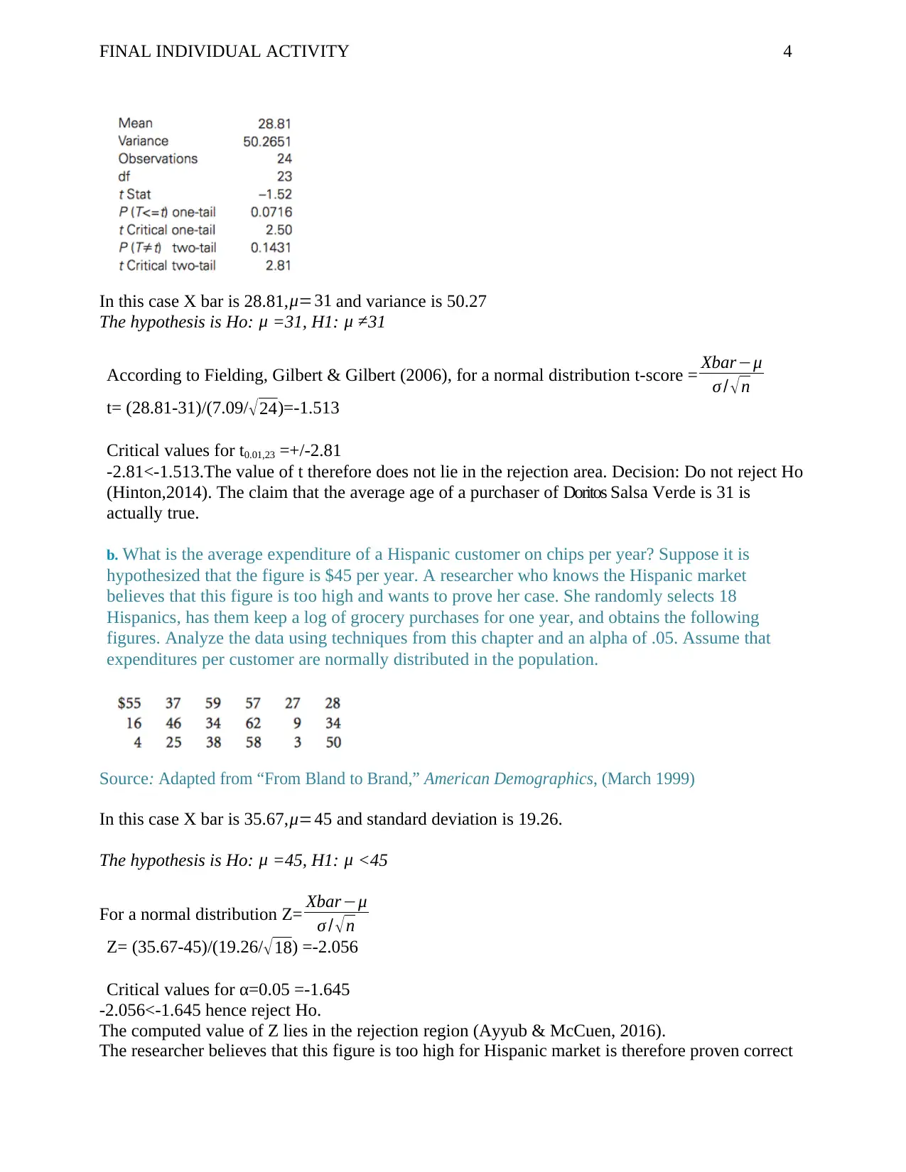
a. What is the average age of a purchaser of Doritos Salsa Verde? Suppose initial tests indicate
that the mean age is 31. Is this figure really correct? To test whether it is, a researcher randomly
contacts 24 purchasers of Doritos Salsa Verde with results shown in the following Excel
output. Discuss the output in terms of a hypothesis test to determine whether the mean age is
actually 31. Let 𝛼 be .01. Assume that ages of purchasers are normally distributed in the
population.

FINAL INDIVIDUAL ACTIVITY 4
In this case X bar is 28.81, μ=31 and variance is 50.27
The hypothesis is Ho: μ =31, H1: μ ≠31
According to Fielding, Gilbert & Gilbert (2006), for a normal distribution t-score = Xbar−μ
σ / √ n
t= (28.81-31)/(7.09/ √24)=-1.513
Critical values for t0.01,23 =+/-2.81
-2.81<-1.513.The value of t therefore does not lie in the rejection area. Decision: Do not reject Ho
(Hinton,2014). The claim that the average age of a purchaser of Doritos Salsa Verde is 31 is
actually true.
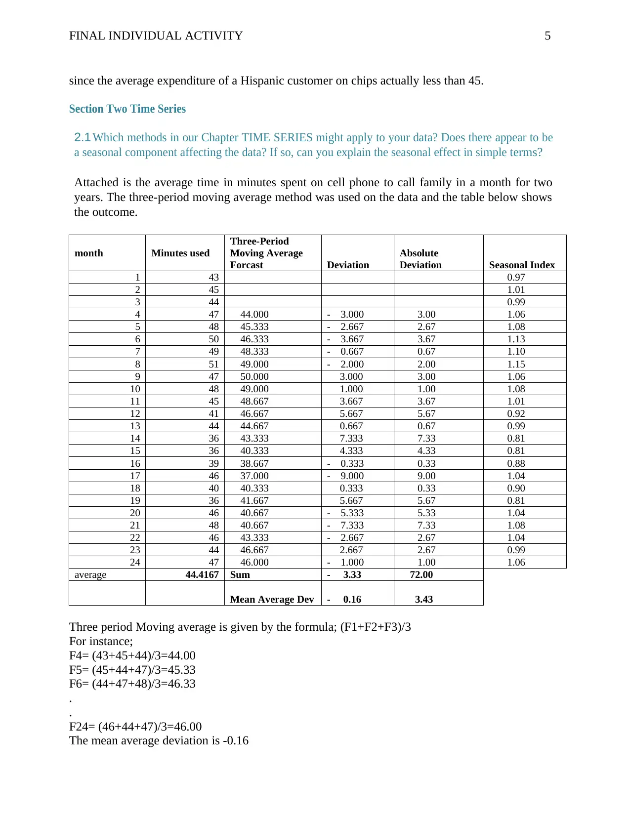
b. What is the average expenditure of a Hispanic customer on chips per year? Suppose it is
hypothesized that the figure is $45 per year. A researcher who knows the Hispanic market
believes that this figure is too high and wants to prove her case. She randomly selects 18
Hispanics, has them keep a log of grocery purchases for one year, and obtains the following
figures. Analyze the data using techniques from this chapter and an alpha of .05. Assume that
expenditures per customer are normally distributed in the population.
Source : Adapted from “From Bland to Brand,” American Demographics, (March 1999)
In this case X bar is 35.67,μ=45 and standard deviation is 19.26.
The hypothesis is Ho: μ =45, H1: μ <45
For a normal distribution Z= Xbar−μ
σ / √n
Z= (35.67-45)/(19.26/√18) =-2.056
Critical values for α=0.05 =-1.645
-2.056<-1.645 hence reject Ho.
The computed value of Z lies in the rejection region (Ayyub & McCuen, 2016).
The researcher believes that this figure is too high for Hispanic market is therefore proven correct

FINAL INDIVIDUAL ACTIVITY 5
since the average expenditure of a Hispanic customer on chips actually less than 45.
Section Two Time Series
2.1 Which methods in our Chapter TIME SERIES might apply to your data? Does there appear to be
a seasonal component affecting the data? If so, can you explain the seasonal effect in simple terms?
Attached is the average time in minutes spent on cell phone to call family in a month for two
years. The three-period moving average method was used on the data and the table below shows
the outcome.
month Minutes used
Three-Period
Moving Average
Forcast Deviation
Absolute
Deviation Seasonal Index
1 43 0.97
2 45 1.01
3 44 0.99
4 47 44.000 - 3.000 3.00 1.06
5 48 45.333 - 2.667 2.67 1.08
6 50 46.333 - 3.667 3.67 1.13
7 49 48.333 - 0.667 0.67 1.10
8 51 49.000 - 2.000 2.00 1.15
9 47 50.000 3.000 3.00 1.06
10 48 49.000 1.000 1.00 1.08
11 45 48.667 3.667 3.67 1.01
12 41 46.667 5.667 5.67 0.92
13 44 44.667 0.667 0.67 0.99
14 36 43.333 7.333 7.33 0.81
15 36 40.333 4.333 4.33 0.81
16 39 38.667 - 0.333 0.33 0.88
17 46 37.000 - 9.000 9.00 1.04
18 40 40.333 0.333 0.33 0.90
19 36 41.667 5.667 5.67 0.81
20 46 40.667 - 5.333 5.33 1.04
21 48 40.667 - 7.333 7.33 1.08
22 46 43.333 - 2.667 2.67 1.04
23 44 46.667 2.667 2.67 0.99
24 47 46.000 - 1.000 1.00 1.06
average 44.4167 Sum - 3.33 72.00
Mean Average Dev - 0.16 3.43
Three period Moving average is given by the formula; (F1+F2+F3)/3
For instance;
F4= (43+45+44)/3=44.00
F5= (45+44+47)/3=45.33
F6= (44+47+48)/3=46.33
.
.
F24= (46+44+47)/3=46.00
The mean average deviation is -0.16

FINAL INDIVIDUAL ACTIVITY 6
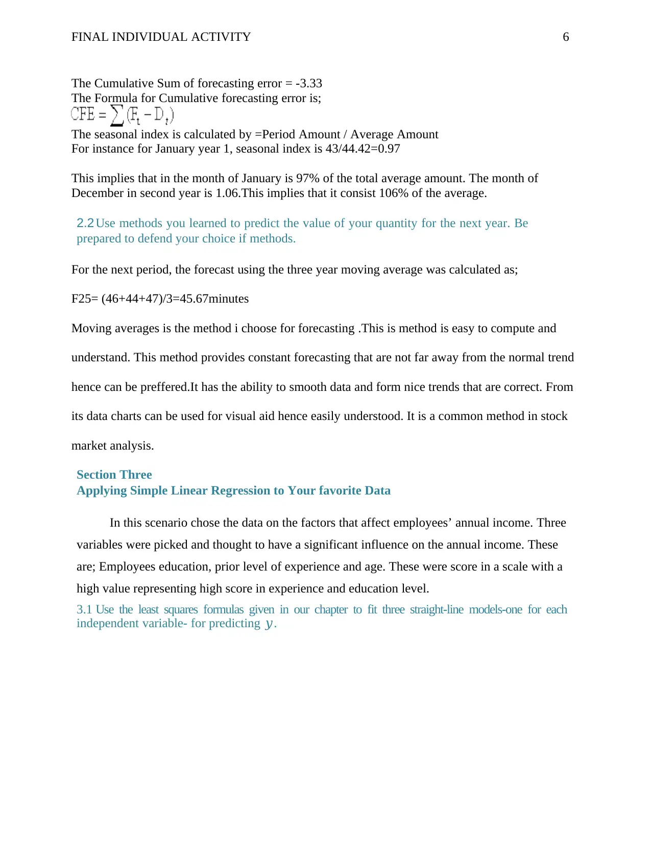
The Cumulative Sum of forecasting error = -3.33
The Formula for Cumulative forecasting error is;
The seasonal index is calculated by =Period Amount / Average Amount
For instance for January year 1, seasonal index is 43/44.42=0.97
This implies that in the month of January is 97% of the total average amount. The month of
December in second year is 1.06.This implies that it consist 106% of the average.
2.2 Use methods you learned to predict the value of your quantity for the next year. Be
prepared to defend your choice if methods.
For the next period, the forecast using the three year moving average was calculated as;
F25= (46+44+47)/3=45.67minutes
Moving averages is the method i choose for forecasting .This is method is easy to compute and
understand. This method provides constant forecasting that are not far away from the normal trend
hence can be preffered.It has the ability to smooth data and form nice trends that are correct. From
its data charts can be used for visual aid hence easily understood. It is a common method in stock
market analysis.
Section Three
Applying Simple Linear Regression to Your favorite Data
In this scenario chose the data on the factors that affect employees’ annual income. Three
variables were picked and thought to have a significant influence on the annual income. These
are; Employees education, prior level of experience and age. These were score in a scale with a
high value representing high score in experience and education level.
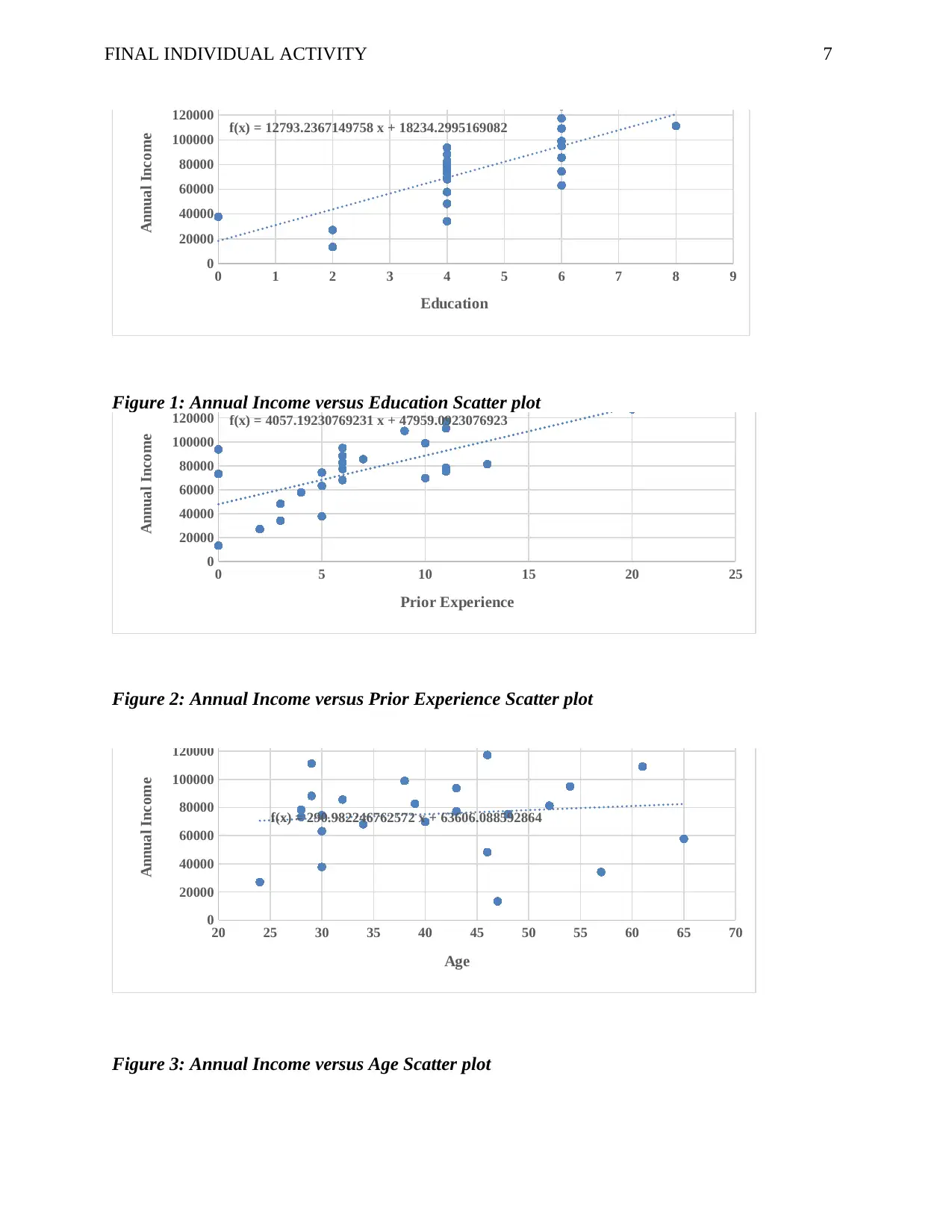
3.1 Use the least squares formulas given in our chapter to fit three straight-line models-one for each
independent variable- for predicting 𝑦.

FINAL INDIVIDUAL ACTIVITY 7
0 1 2 3 4 5 6 7 8 9
0
20000
40000
60000
80000
100000
120000
140000
f(x) = 12793.2367149758 x + 18234.2995169082
Income versus Education
Education
Annual Income
Figure 1: Annual Income versus Education Scatter plot
0 5 10 15 20 25
0
20000
40000
60000
80000
100000
120000
140000
f(x) = 4057.19230769231 x + 47959.0923076923
Annual income vs Prior Experience
Prior Experience
Annual Income
Figure 2: Annual Income versus Prior Experience Scatter plot
20 25 30 35 40 45 50 55 60 65 70
0
20000
40000
60000
80000
100000
120000
140000
f(x) = 290.982246762572 x + 63606.088592864
Annual income vs Age
Age
Annual Income
Figure 3: Annual Income versus Age Scatter plot

1
FINAL INDIVIDUAL ACTIVITY 8
Education Regression equation; y = 12793x + 18234
Prior Experience Regression equation y = 4057.2x + 47959
Age Regression equation y = 290.98x + 63606
3.2 In ter pr et th e s ig n of the es tim ated s lo p e coefficient 𝛽̂ in each case, and test the utility of each
model by testing 𝐻0: 𝛽1 = 0 against 𝐻𝑎: 𝛽1 ≠ 0. What assumptions must be satisfied to ensure the
validity of these tests?
The coefficient of education is positive. This implies that there is a positive relationship between annual
income and education. As the level of education increases, the annual income increased and vice versa.
The coefficient of prior experience is positive. This implies that there is a positive relationship between annual
income and prior experience. As prior experience increases, the annual income increases and vice versa.
The coefficient of age is positive. This implies that there is a positive relationship between annual income and
age. As age increased, the annual income increased and vice versa.
a). For First variable independent variable; education; y = 12793x + 18234
Standard error (error term) e =2324.53, 11079.99
Step 1: Statistical significance test for x
H0: β1 = 0
H1: β1≠ 0
Step 2 = β 1−0
S β = 12793−0
2324.53 =5.504
Step 3: Decision at 5% level of significance, critical value is +/-1.96 (King’oriah, 2014).
Since 5.504>1.96 at 5% we reject the null hypothesis and conclude that education has a statistically
significant influence on the respondents annual income.
b). For second independent variable; prior experience; y = 4057.2x + 47959
Standard error (error term) e =937.6, 7676.86
Step 1: Statistical significance test for x
H0: β1 = 0
H1: β1≠ 0
Step 2 = β 1−0
S β = 4057.2−0
937.6 =4.33
Step 3: Decision at 5% level of significance, critical value is +/-1.96
Since 4.33 >1.96 at 5% we reject the null hypothesis and conclude that prior experience has a
statistically significant influence on the respondents annual income (Larson & Farber, 2019)

FINAL INDIVIDUAL ACTIVITY 9
c). For third independent variable ‘age; y = 290.98x + 63606
Standard error (error term) e =209.98, 502.98
Step 1: Statistical significance test for x
H0: β1 = 0
H1: β1≠ 0
Step 2 = β 1−0
S β = 290.98−0
502.98 =0.579
Step 3: Decision at 5% level of significance, critical value is +/-1.96
Since 0.579<1.96 at 5% we do not reject the null hypothesis and conclude that age has no
statistically significant influence on the respondents annual income.
According to Berenson, Timothy, David M.(2005) the following are some of the assumption of the
regression model.
Assumptions
 The errors are normally distributed
 The observation are independent
 Homoscedasticity of errors (Equality of variance).
 The model has a linear relationship
3.3 Calculate the coefficient of determination, 𝑟 2 , for each model. Which of the independent
variables predicts 𝑦 best for the 25 sampled sets of data? Is this variable necessarily best in
general (i.e., for the entire population)? Explain.
Regression Statistics Education Prior Experience Age
Multiple R 0.754 0.670 0.120
R Square 0.568 0.449 0.014
Adjusted R Square 0.550 0.425 -0.029
Standard Error 18918.87 21380.53 28590.04
Observations 25 25 25
For the independent variable education; R2 =0.568.This implies that the variable explains
56.8% of the variation in the model. The independent variable prior experience has R2 =0.449.This
implies that the variable explains 44.9% of the variation in the model. Also, Age model had a R2

FINAL INDIVIDUAL ACTIVITY 10
=0.014,which implies that 1.4% of the variation is explained by the model (Elliott, Gargano, &
Timmermann, 2013).
Considering their R-squared values for the three variables, the level of education is the best
predictor of the variable income (56.8%).It also has a significant influence on annual income
(p<.05).When all the other factors are included in the model,education still is the best predictor in
the model ;Annual Income=9619.9Education+2513.2Prior experience-38.63 Age+16946.5.
References
Ayyub, B. M., & McCuen, R. H. (2016). Probability, statistics, and reliability for engineers and scientists.
CRC press.
Berenson, M. L., Timothy, C. K., David M. L. (2005). Basic business statistics: concepts and applications.
10th ed. New York, NY: Prentice Hall.
Coladarci, T. & Cobb, C. (2013) Fundamentals of Statistical Reasoning in Education, 4th ed. Hoboken,
New Jersey Wiley & Sons.
Elliott, G., Gargano, A., & Timmermann, A. (2013). Complete subset regressions. Journal of
Econometrics, 177(2), 357-373.
Fielding, J., Gilbert, N., & Gilbert, G. N. (2006). Understanding social statistics. California: SAGE
Publications.
Hinton, P. R. (2014). Statistics explained. Routledge.
King’oriah, G. K. (2014). Fundamentals of applied statistics. Nairobi: Jomo Kenyatta
Larson, R., & Farber, B. (2019). Elementary statistics. Pearson.
Source : Adapted from “From Bland to Brand,” American Demographics, (March 1999), p. 57; Ronald
J. Alsop, ed., The Wall Street Journal Almanac 1999. New York: Ballantine Books, 1998, p.
202; and the 2008 Frito-Lay Web site at http://www.fritolay.com/index.html