Financial Management and Decision Making: Investment Analysis
VerifiedAdded on 2023/06/07
|15
|1608
|399
Homework Assignment
AI Summary
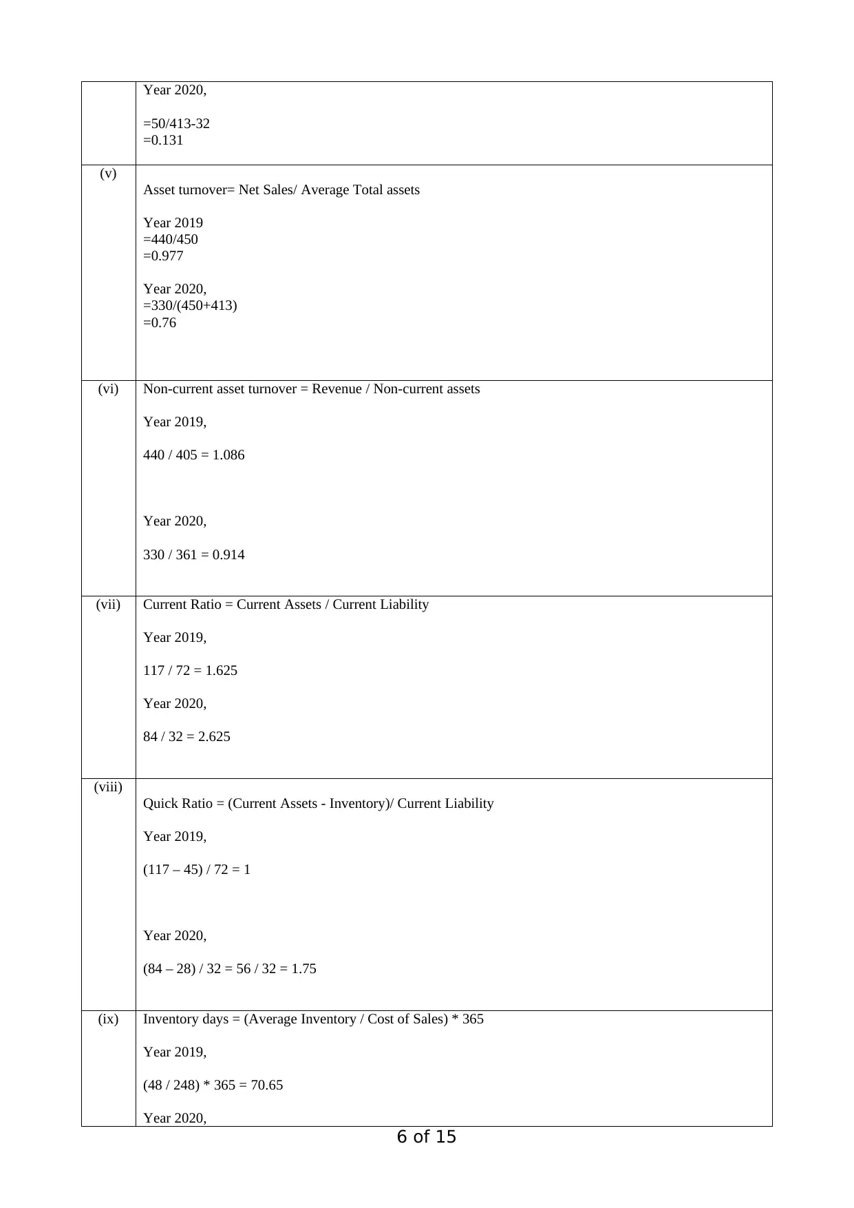
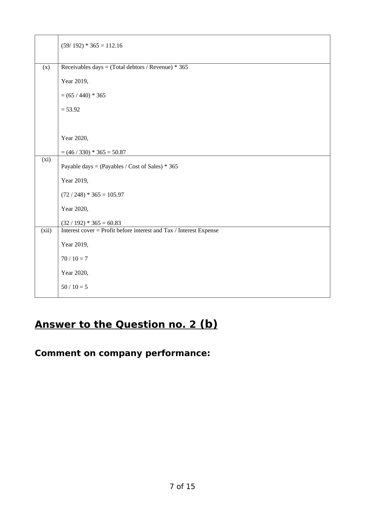
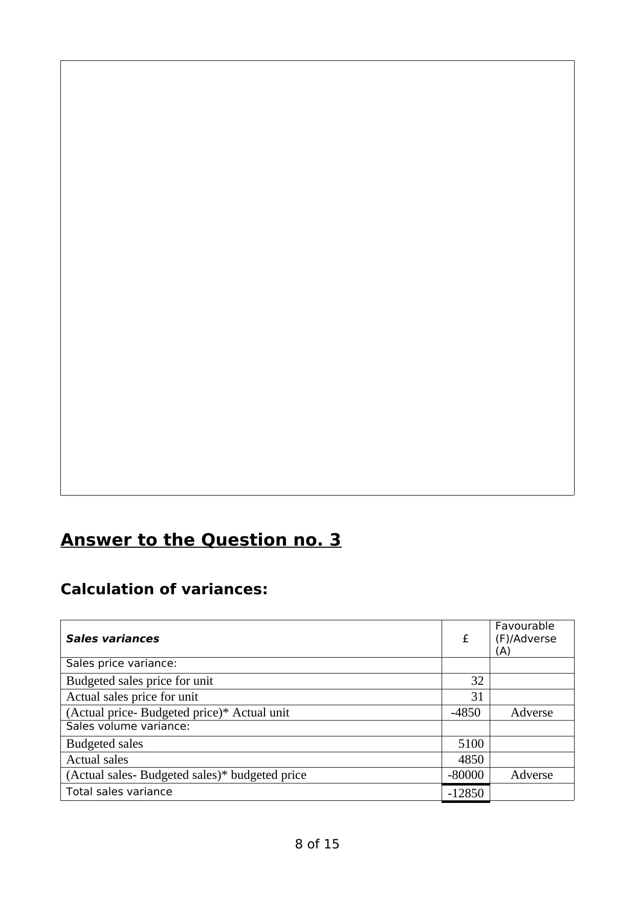
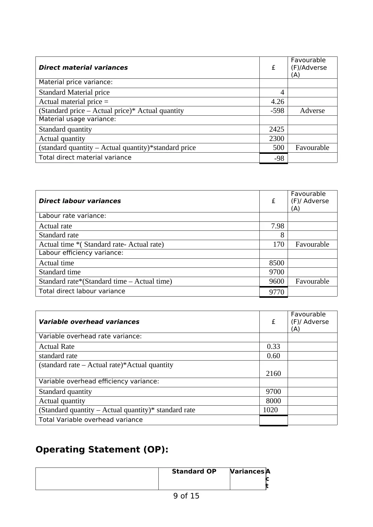
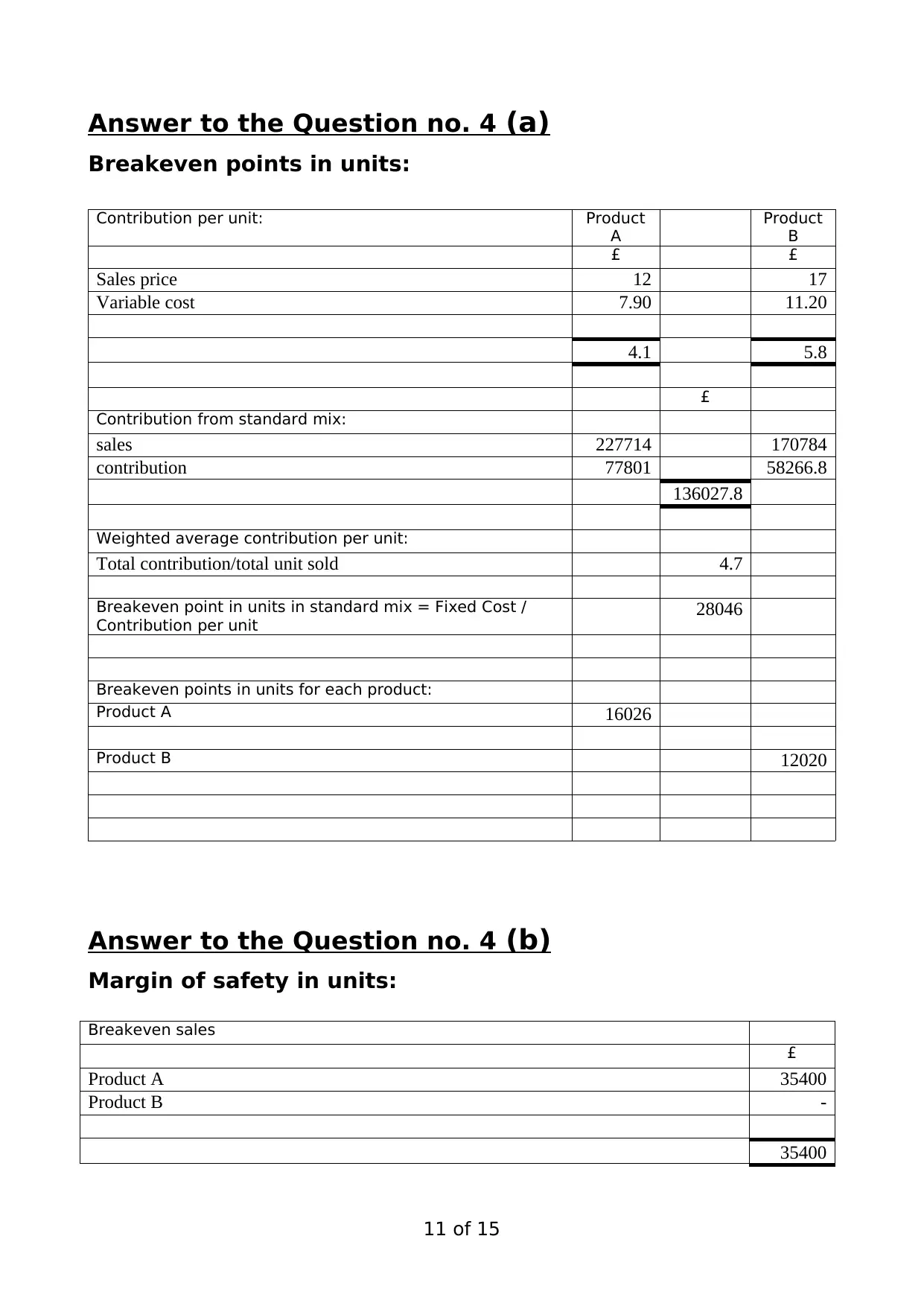
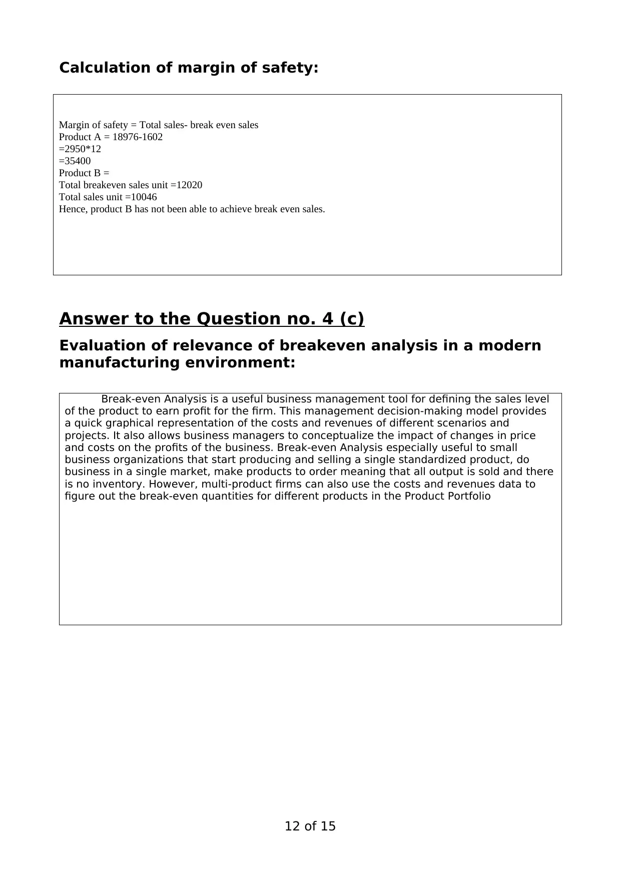
This assignment solution for a Financial Management module (BMP5006) includes detailed calculations and analysis of investment projects using payback period and Net Present Value (NPV) methods, along with a comparative assessment of project viability. It also covers financial ratio analysis, including gross profit ratio, operating profit ratio, and asset turnover, to evaluate company performance across two years. Furthermore, the assignment addresses variance analysis for sales, direct materials, and direct labor, providing a comprehensive operating statement. Finally, it includes break-even analysis, margin of safety calculations, and an evaluation of the relevance of break-even analysis in modern manufacturing, concluding with significant steps in setting a financial/cost controlling budget in a large organisation. Desklib provides students access to this and many other solved assignments.


1 out of 15
Related Documents


Your All-in-One AI-Powered Toolkit for Academic Success.
+13062052269
info@desklib.com
Available 24*7 on WhatsApp / Email
![[object Object]](/_next/static/media/star-bottom.7253800d.svg)
Copyright © 2020–2026 A2Z Services. All Rights Reserved. Developed and managed by ZUCOL.