Solution to Homework on Fixed Income Securities & Derivatives Pricing

This document presents a detailed solution to a homework assignment focused on fixed income securities and derivatives pricing. The solution covers various aspects, including constructing interest rate trees using the BDT model, valuing callable bonds, and applying Monte Carlo simulations for pricing securities. Specific exercises address topics such as calculating zero-coupon bond prices, determining option values in callable bonds, and analyzing mortgage-backed securities. The document also compares results obtained through risk-neutral pricing and Monte Carlo simulation methods, highlighting the accuracy and convergence of these approaches. Additionally, it includes calculations for bond duration and convexity, as well as the derivation of implied interest rates from bond prices and forward rate agreements. This comprehensive solution provides valuable insights into the practical application of fixed income and derivatives pricing models.

Exercise 1
Part 1
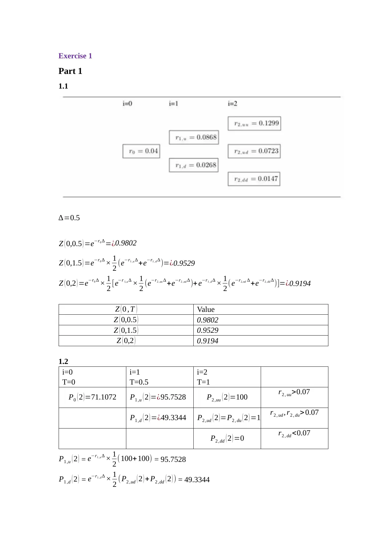
1.1
∆=0.5
Z ( 0,0.5 ) =e−r0 ∆ =¿0.9802
Z ( 0,1.5 ) =e−r0 ∆ × 1
2 (e−r1 ,u ∆ +e−r1 ,d ∆ )=¿0.9529
Z ( 0,2 ) =e−r0 ∆ × 1
2 [e−r 1,u ∆ × 1
2 (e−r2 ,uu ∆ +e−r2 ,ud ∆ )+e−r1 ,d ∆ × 1
2 (e−r2,ud ∆ +e−r2 ,dd ∆ )]=¿0.9194
Z ( 0 , T ) Value
Z ( 0,0.5 ) 0.9802
Z ( 0,1.5 ) 0.9529
Z ( 0,2 ) 0.9194
1.2
i=0 i=1 i=2
T=0 T=0.5 T=1
P0 ( 2 )=71.1072 P1 ,u ( 2 )=¿95.7528 P2 ,uu ( 2 )=100 r2 , uu>0.07
P1 ,d ( 2 ) =¿49.3344 P2 ,ud ( 2 ) =P2 , du ( 2 ) =100 r2 , ud , r2 , du> 0.07
P2 ,dd ( 2 ) =0 r2 , dd <0.07
P1 ,u ( 2 ) = e−r1 ,u ∆ × 1
2 (100+100) = 95.7528
P1 ,d ( 2 ) = e−r1 ,d ∆ × 1
2 (P2 ,ud ( 2 ) + P2 ,dd ( 2 ) ) = 49.3344

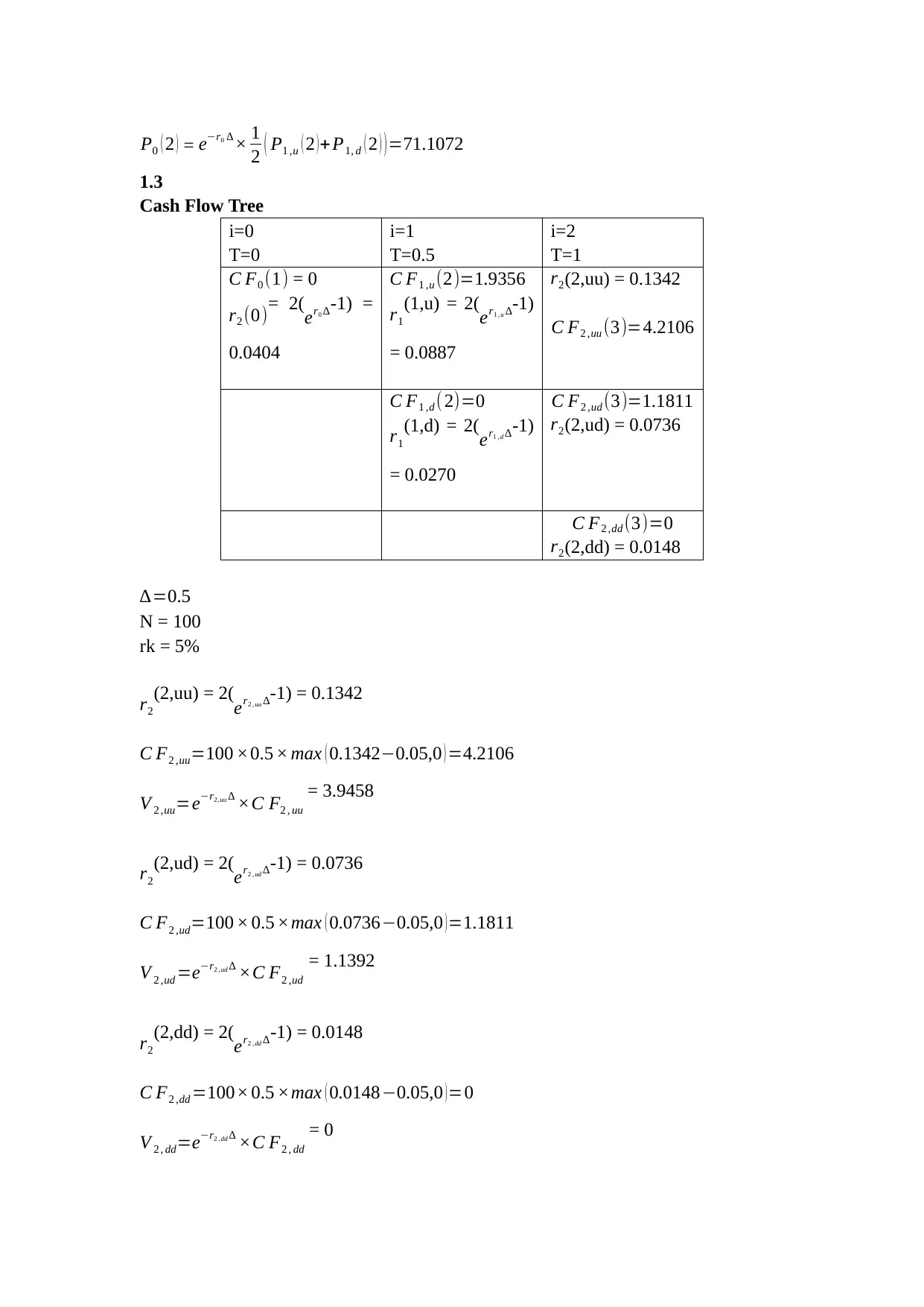
P0 ( 2 ) = e−r0 ∆ × 1
2 ( P1 ,u ( 2 ) +P1, d ( 2 ) ) =71.1072
1.3
Cash Flow Tree
i=0 i=1 i=2
T=0 T=0.5 T=1
C F0 (1) = 0
r2 (0)= 2(er0 ∆-1) =
0.0404
C F1 ,u (2)=1.9356
r1
(1,u) = 2(
er1 , u ∆-1)
= 0.0887
r2(2,uu) = 0.1342
C F2 ,uu (3)=4.2106
C F1 ,d ( 2)=0
r1
(1,d) = 2(er1 ,d ∆-1)
= 0.0270
C F2 ,ud (3)=1.1811
r2(2,ud) = 0.0736
C F2 ,dd (3)=0
r2(2,dd) = 0.0148
∆=0.5
N = 100
rk = 5%
r2
(2,uu) = 2(
er2 , uu ∆-1) = 0.1342
C F2 ,uu=100 ×0.5 × max ( 0.1342−0.05,0 ) =4.2106
V 2 ,uu=e−r2,uu ∆ ×C F2 , uu
= 3.9458
r2
(2,ud) = 2(er2 ,ud ∆-1) = 0.0736
C F2 ,ud=100 × 0.5 ×max ( 0.0736−0.05,0 ) =1.1811
V 2 ,ud =e−r2 ,ud ∆ ×C F2 ,ud
= 1.1392
r2
(2,dd) = 2(er2 ,dd ∆-1) = 0.0148
C F2 ,dd =100× 0.5 ×max ( 0.0148−0.05,0 ) =0
V 2 , dd=e−r2 ,dd ∆ ×C F2 , dd
= 0

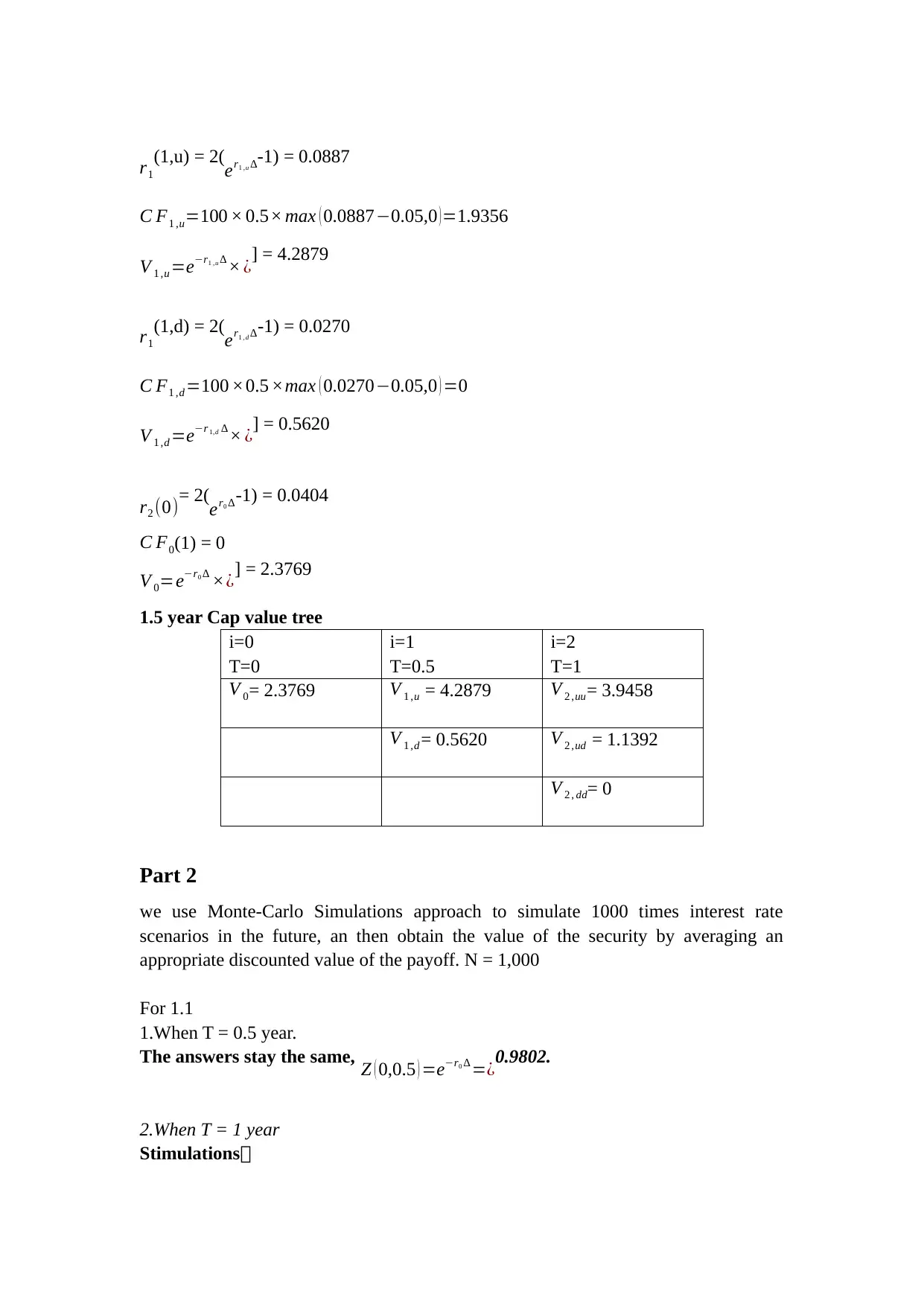
r1
(1,u) = 2(
er1 ,u ∆-1) = 0.0887
C F1 ,u=100 × 0.5× max ( 0.0887−0.05,0 ) =1.9356
V 1 ,u =e−r1 ,u ∆ × ¿] = 4.2879
r1
(1,d) = 2(er1 ,d ∆-1) = 0.0270
C F1 ,d =100 ×0.5 ×max ( 0.0270−0.05,0 ) =0
V 1 ,d =e−r 1,d ∆ × ¿] = 0.5620
r2 (0)= 2(
er0 ∆-1) = 0.0404
C F0(1) = 0
V 0=e−r0 ∆ ׿] = 2.3769
1.5 year Cap value tree
i=0 i=1 i=2
T=0 T=0.5 T=1
V 0= 2.3769 V 1 ,u = 4.2879 V 2 ,uu= 3.9458
V 1 ,d = 0.5620 V 2 ,ud = 1.1392
V 2 , dd= 0
Part 2
we use Monte-Carlo Simulations approach to simulate 1000 times interest rate
scenarios in the future, an then obtain the value of the security by averaging an
appropriate discounted value of the payoff. N = 1,000
For 1.1
1.When T = 0.5 year.
The answers stay the same, Z ( 0,0.5 ) =e−r0 ∆ =¿0.9802.
2.When T = 1 year
Stimulations：

In this way, we obtain the average payoff ^c0
= 1
1000 ∑
s=1
1000
e−r0 ×0.5 × c1
s = 95.3031
Z(0,1) = ^c0 / 100 = 0.9530
Standard error = 0.045189
Confidence interval = [ 95.21272, 95.39348]
3.When T = 1.5 year
Stimulations：
In this way, we obtain the average payoff ^c0
= 1
1000 ∑
s=1
1000
e−(r0+ r1
s )× 0.5× c2
s = 91.8938
Z(0,1.5) = ^c0 / 100 = 0.9189
Standard error = 0.095118
Confidence interval = [91.70356,92.08404]
For 1.2
Stimulations：

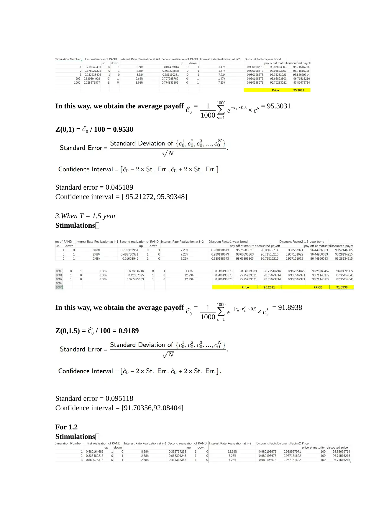
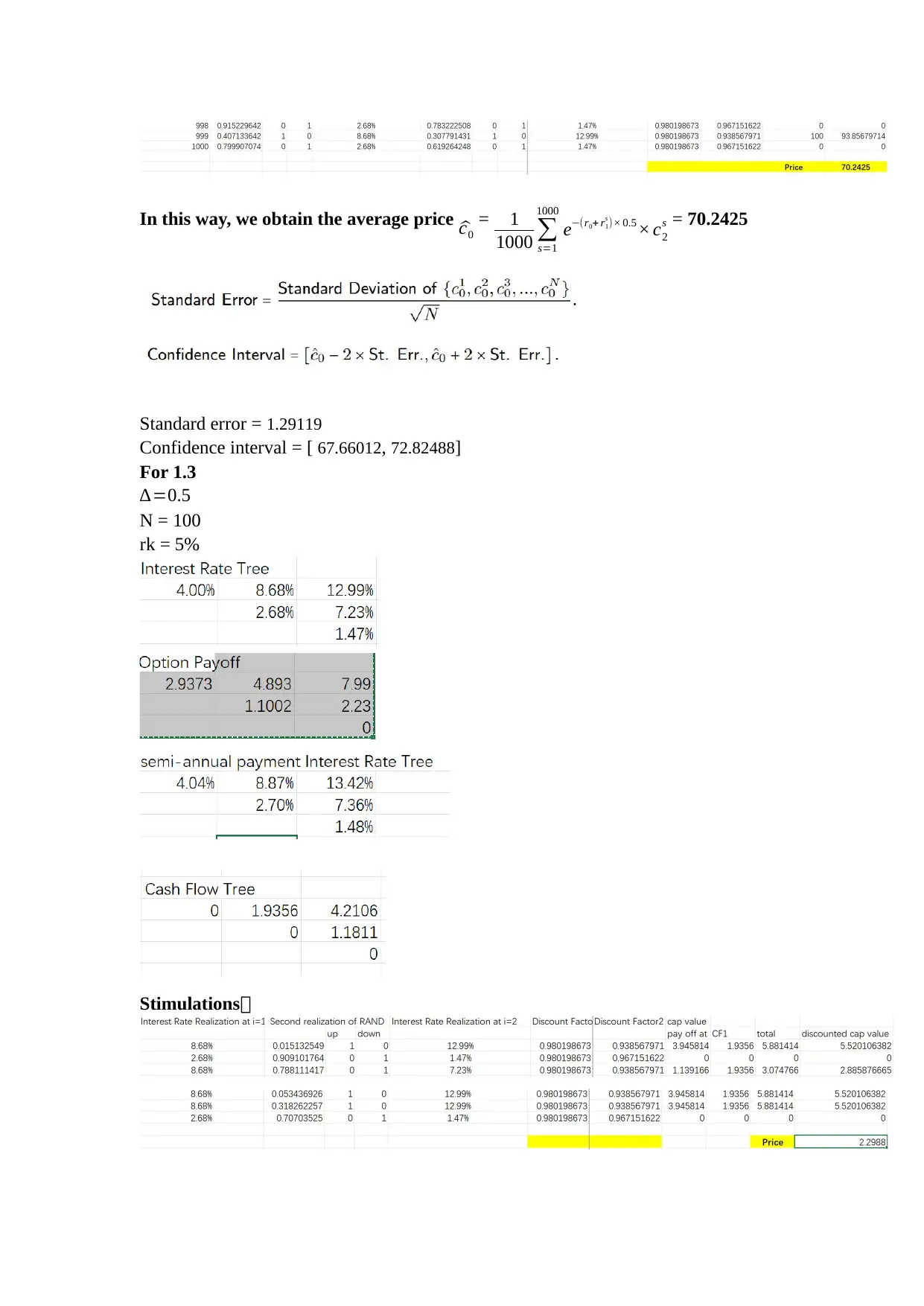
In this way, we obtain the average price ^c0
= 1
1000 ∑
s=1
1000
e−(r0+ r1
s )× 0.5 × c2
s = 70.2425
Standard error = 1.29119
Confidence interval = [ 67.66012, 72.82488]
For 1.3
∆=0.5
N = 100
rk = 5%
Stimulations：

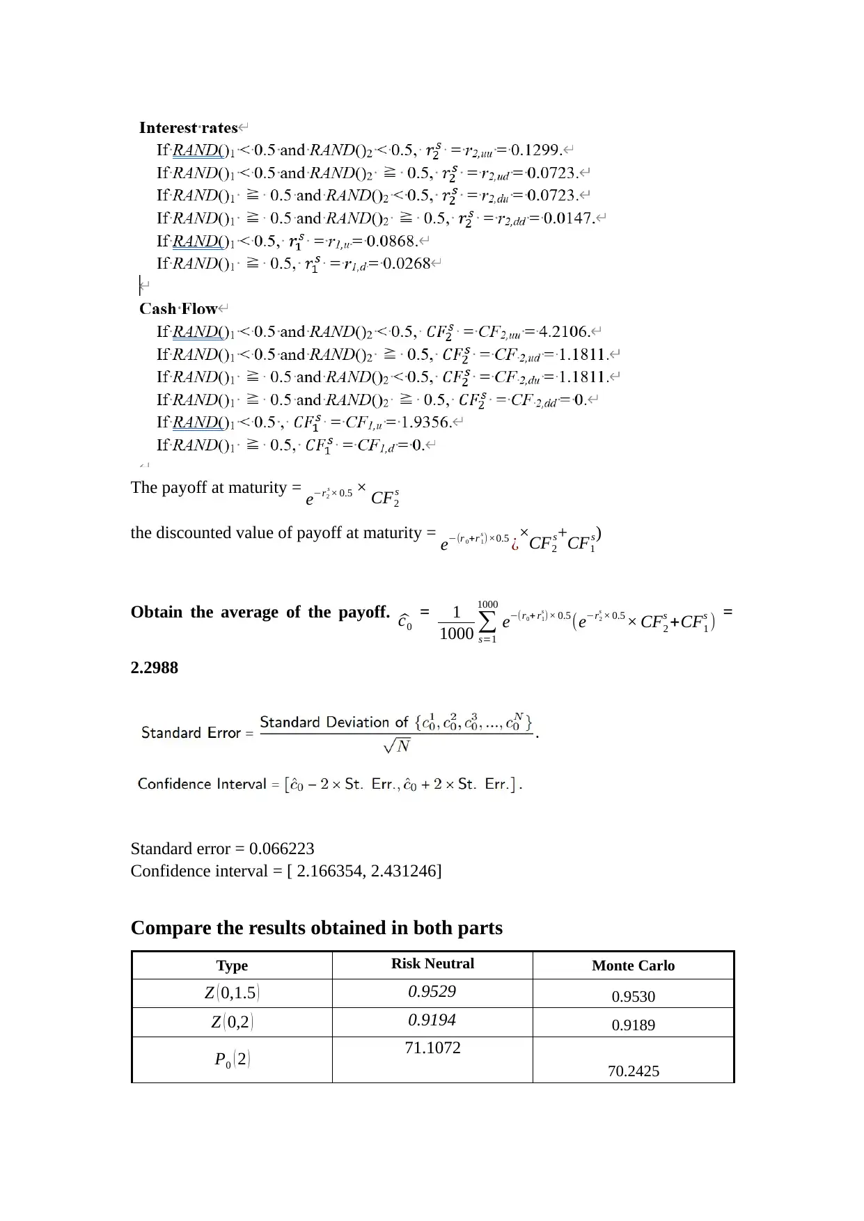
The payoff at maturity = e−r2
s × 0.5 × CF2
s
the discounted value of payoff at maturity = e−(r 0+r 1
s )×0.5 ¿×
CF2
s+CF1
s)
Obtain the average of the payoff. ^c0
= 1
1000 ∑
s=1
1000
e−(r0+ r1
s )× 0.5(e−r2
s × 0.5× CF2
s +CF1
s ) =
2.2988
Standard error = 0.066223
Confidence interval = [ 2.166354, 2.431246]
Compare the results obtained in both parts
Type Risk Neutral Monte Carlo
Z ( 0,1.5 ) 0.9529 0.9530
Z ( 0,2 ) 0.9194 0.9189
P0 ( 2 ) 71.1072
70.2425

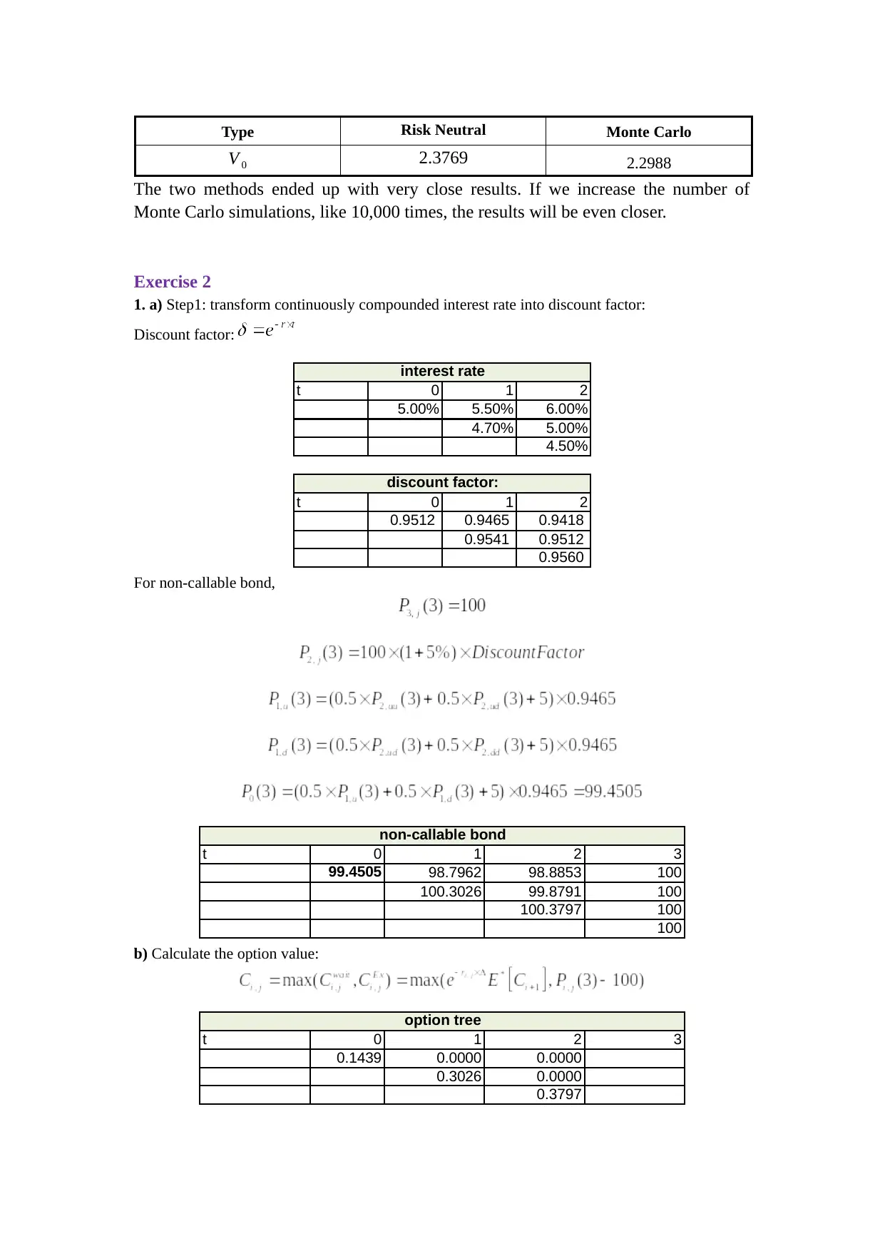
Type Risk Neutral Monte Carlo
V 0 2.3769 2.2988
The two methods ended up with very close results. If we increase the number of
Monte Carlo simulations, like 10,000 times, the results will be even closer.
Exercise 2
1. a) Step1: transform continuously compounded interest rate into discount factor:
Discount factor:
interest rate non-c
t 0 1 2
5.00% 5.50% 6.00%
4.70% 5.00%
4.50%
discount factor:
t 0 1 2
0.9512 0.9465 0.9418
0.9541 0.9512
0.9560
For non-callable bond,
non-callable bond
t 0 1 2 3
99.4505 98.7962 98.8853 100
100.3026 99.8791 100
100.3797 100
100
b) Calculate the option value:
option tree
t 0 1 2 3
0.1439 0.0000 0.0000
0.3026 0.0000
0.3797

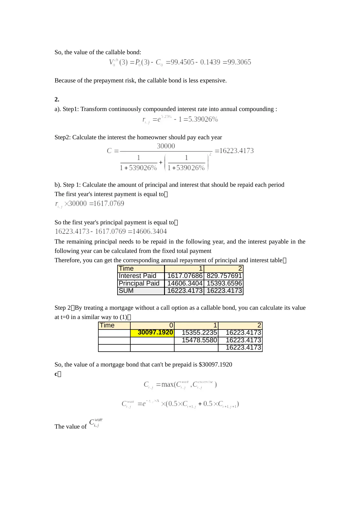
So, the value of the callable bond:
Because of the prepayment risk, the callable bond is less expensive.
2.
a). Step1: Transform continuously compounded interest rate into annual compounding :
Step2: Calculate the interest the homeowner should pay each year
b). Step 1: Calculate the amount of principal and interest that should be repaid each period
The first year's interest payment is equal to：
So the first year's principal payment is equal to：
The remaining principal needs to be repaid in the following year, and the interest payable in the
following year can be calculated from the fixed total payment
Therefore, you can get the corresponding annual repayment of principal and interest table：
Time 1 2
Interest Paid 1617.07686 829.757691
Principal Paid 14606.3404 15393.6596
SUM 16223.4173 16223.4173
Step 2：By treating a mortgage without a call option as a callable bond, you can calculate its value
at t=0 in a similar way to (1)：
Time 0 1 2
30097.1920 15355.2235 16223.4173
15478.5580 16223.4173
16223.4173
So, the value of a mortgage bond that can't be prepaid is $30097.1920
c：
The value of

Time 0 1 2
40.3789 0 0
0 0
0
Time 0 1 2
97.1920 0 0
84.8984 0
0
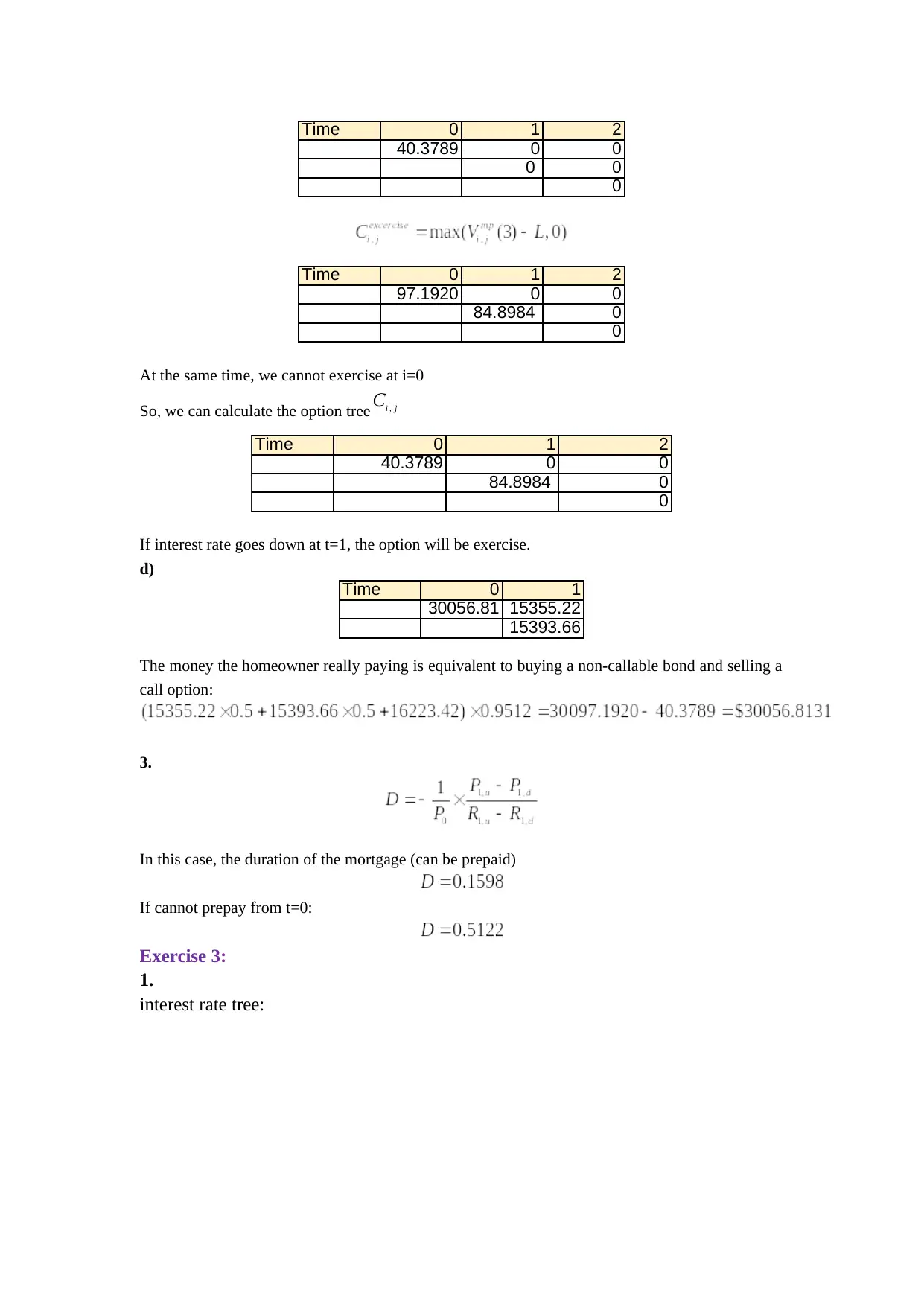
At the same time, we cannot exercise at i=0
So, we can calculate the option tree
Time 0 1 2
40.3789 0 0
84.8984 0
0
If interest rate goes down at t=1, the option will be exercise.
d)
Time 0 1
30056.81 15355.22
15393.66
The money the homeowner really paying is equivalent to buying a non-callable bond and selling a
call option:
3.
In this case, the duration of the mortgage (can be prepaid)
If cannot prepay from t=0:
Exercise 3:
1.
interest rate tree:

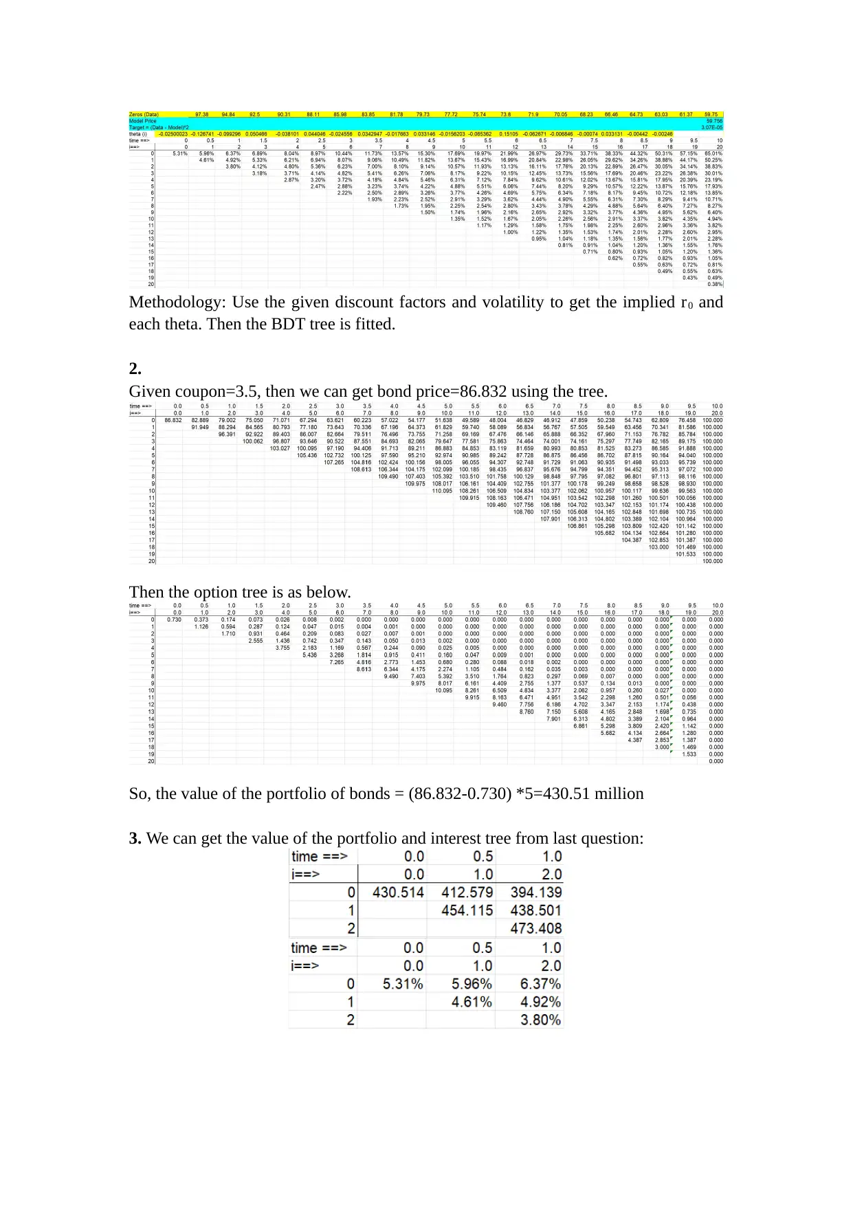
Methodology: Use the given discount factors and volatility to get the implied r0 and
each theta. Then the BDT tree is fitted.
2.
Given coupon=3.5, then we can get bond price=86.832 using the tree.
Then the option tree is as below.
So, the value of the portfolio of bonds = (86.832-0.730) *5=430.51 million
3. We can get the value of the portfolio and interest tree from last question:

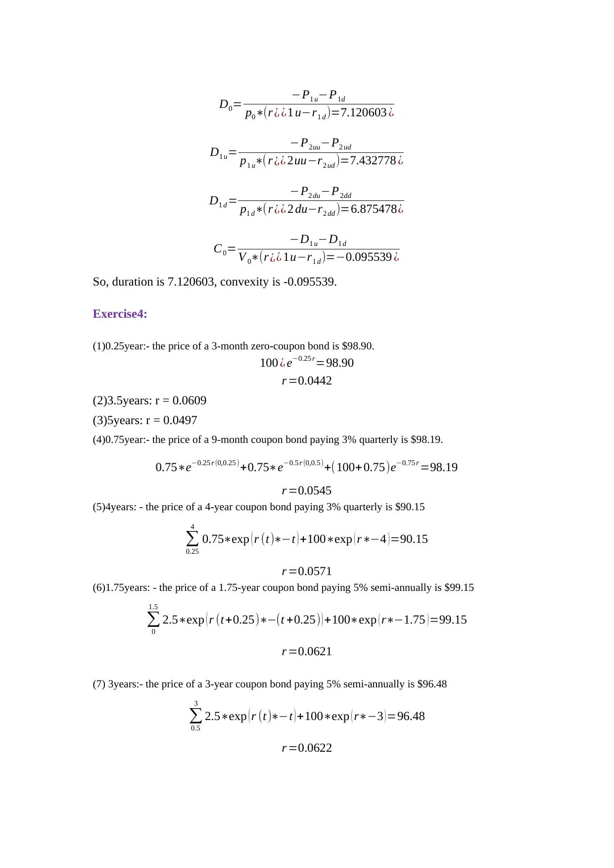
D0= −P1 u−P1d
p0∗(r ¿ ¿1 u−r1 d )=7.120603 ¿
D1 u= −P2uu−P2 ud
p1 u∗( r ¿¿ 2uu−r2 ud )=7.432778 ¿
D1 d = −P2 du−P2dd
p1 d∗(r ¿¿ 2 du−r2 dd )=6.875478¿
C0= −D1 u−D1 d
V 0∗(r ¿¿ 1u−r1 d )=−0.095539 ¿
So, duration is 7.120603, convexity is -0.095539.
Exercise4:
(1)0.25year:- the price of a 3-month zero-coupon bond is $98.90.
100 ¿ e−0.25 r=98.90
r =0.0442
(2)3.5years: r = 0.0609
(3)5years: r = 0.0497
(4)0.75year:- the price of a 9-month coupon bond paying 3% quarterly is $98.19.
0.75∗e−0.25 r (0,0.25 )+0.75∗e−0.5 r (0,0.5)+(100+0.75)e−0.75 r =98.19
r =0.0545
(5)4years: - the price of a 4-year coupon bond paying 3% quarterly is $90.15
∑
0.25
4
0.75∗exp ( r (t)∗−t ) +100∗exp ( r∗−4 ) =90.15
r =0.0571
(6)1.75years: - the price of a 1.75-year coupon bond paying 5% semi-annually is $99.15
∑
0
1.5
2.5∗exp ( r (t+0.25)∗−(t +0.25) ) +100∗exp ( r∗−1.75 )=99.15
r =0.0621
(7) 3years:- the price of a 3-year coupon bond paying 5% semi-annually is $96.48
∑
0.5
3
2.5∗exp ( r (t)∗−t ) +100∗exp ( r∗−3 ) =96.48
r =0.0622

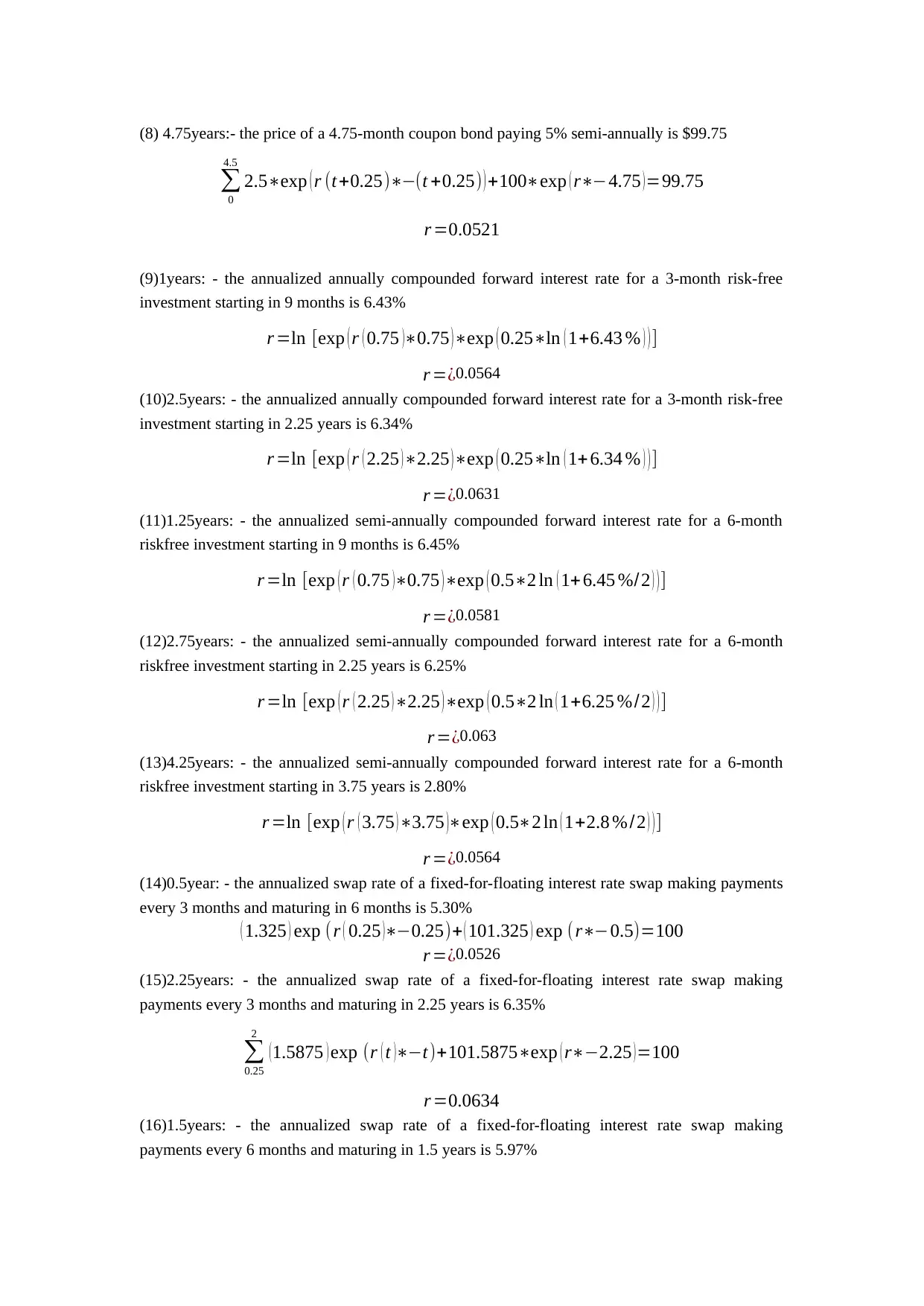
(8) 4.75years:- the price of a 4.75-month coupon bond paying 5% semi-annually is $99.75
∑
0
4.5
2.5∗exp ( r (t+0.25)∗−(t +0.25) ) +100∗exp ( r∗−4.75 )=99.75
r =0.0521
(9)1years: - the annualized annually compounded forward interest rate for a 3-month risk-free
investment starting in 9 months is 6.43%
r =ln [exp ( r ( 0.75 )∗0.75 )∗exp ( 0.25∗ln ( 1+6.43 % ) ) ]
r =¿0.0564
(10)2.5years: - the annualized annually compounded forward interest rate for a 3-month risk-free
investment starting in 2.25 years is 6.34%
r =ln [exp ( r ( 2.25 )∗2.25 )∗exp ( 0.25∗ln ( 1+ 6.34 % ) ) ]
r =¿0.0631
(11)1.25years: - the annualized semi-annually compounded forward interest rate for a 6-month
riskfree investment starting in 9 months is 6.45%
r =ln [exp ( r ( 0.75 )∗0.75 )∗exp ( 0.5∗2 ln ( 1+ 6.45 %/2 ) ) ]
r =¿0.0581
(12)2.75years: - the annualized semi-annually compounded forward interest rate for a 6-month
riskfree investment starting in 2.25 years is 6.25%
r =ln [exp ( r ( 2.25 )∗2.25 )∗exp ( 0.5∗2 ln ( 1+6.25 %/2 ) ) ]
r =¿0.063
(13)4.25years: - the annualized semi-annually compounded forward interest rate for a 6-month
riskfree investment starting in 3.75 years is 2.80%
r =ln [exp ( r ( 3.75 )∗3.75 )∗exp ( 0.5∗2 ln ( 1+2.8 % /2 ) ) ]
r =¿0.0564
(14)0.5year: - the annualized swap rate of a fixed-for-floating interest rate swap making payments
every 3 months and maturing in 6 months is 5.30%
( 1.325 ) exp (r ( 0.25 )∗−0.25)+ ( 101.325 ) exp (r∗−0.5)=100
r =¿0.0526
(15)2.25years: - the annualized swap rate of a fixed-for-floating interest rate swap making
payments every 3 months and maturing in 2.25 years is 6.35%
∑
0.25
2
(1.5875 ) exp (r ( t )∗−t)+101.5875∗exp ( r∗−2.25 )=100
r =0.0634
(16)1.5years: - the annualized swap rate of a fixed-for-floating interest rate swap making
payments every 6 months and maturing in 1.5 years is 5.97%