Financial Modeling: Spreadsheet Model for NPV and IRR
VerifiedAdded on 2023/04/21
|13
|2375
|497
AI Summary
This document provides a step-by-step guide on creating a spreadsheet model to calculate the Net Present Value (NPV) and Internal Rate of Return (IRR) for an investment. It explains the significance of these financial metrics in project evaluation and decision making. The document also includes a sensitivity analysis and correlation analysis to assess the impact of different variables on the project's outcomes.
Contribute Materials
Your contribution can guide someone’s learning journey. Share your
documents today.

FINANCIAL
MODELING
MODELING
Secure Best Marks with AI Grader
Need help grading? Try our AI Grader for instant feedback on your assignments.
TABLE OF CONTENT
INTRODUCTION................................................................................................3
Part 1...............................................................................................................3
Spreadsheet model to find the Net Present Value and Internal rate of
Return for the investment............................................................................3
Part B...............................................................................................................7
Simulation on proposed project....................................................................7
Explanation of what the model is doing..............................................10
Model limitations....................................................................................11
CONCLUSION.................................................................................................11
REFRENCES....................................................................................................12
INTRODUCTION
In today era it is very difficult to make sound business decision. In
order to reduce this complexity simulation methods are used by the
managers. In this report various methods like sensitive analysis and scenario
analysis are done. Along with this project evaluation is also done in the
report. Hence, it can be said that by using these methods best decisions can
be made by the managers.
PART 1
Spreadsheet model to find the Net Present Value and Internal rate of Return
for the investment
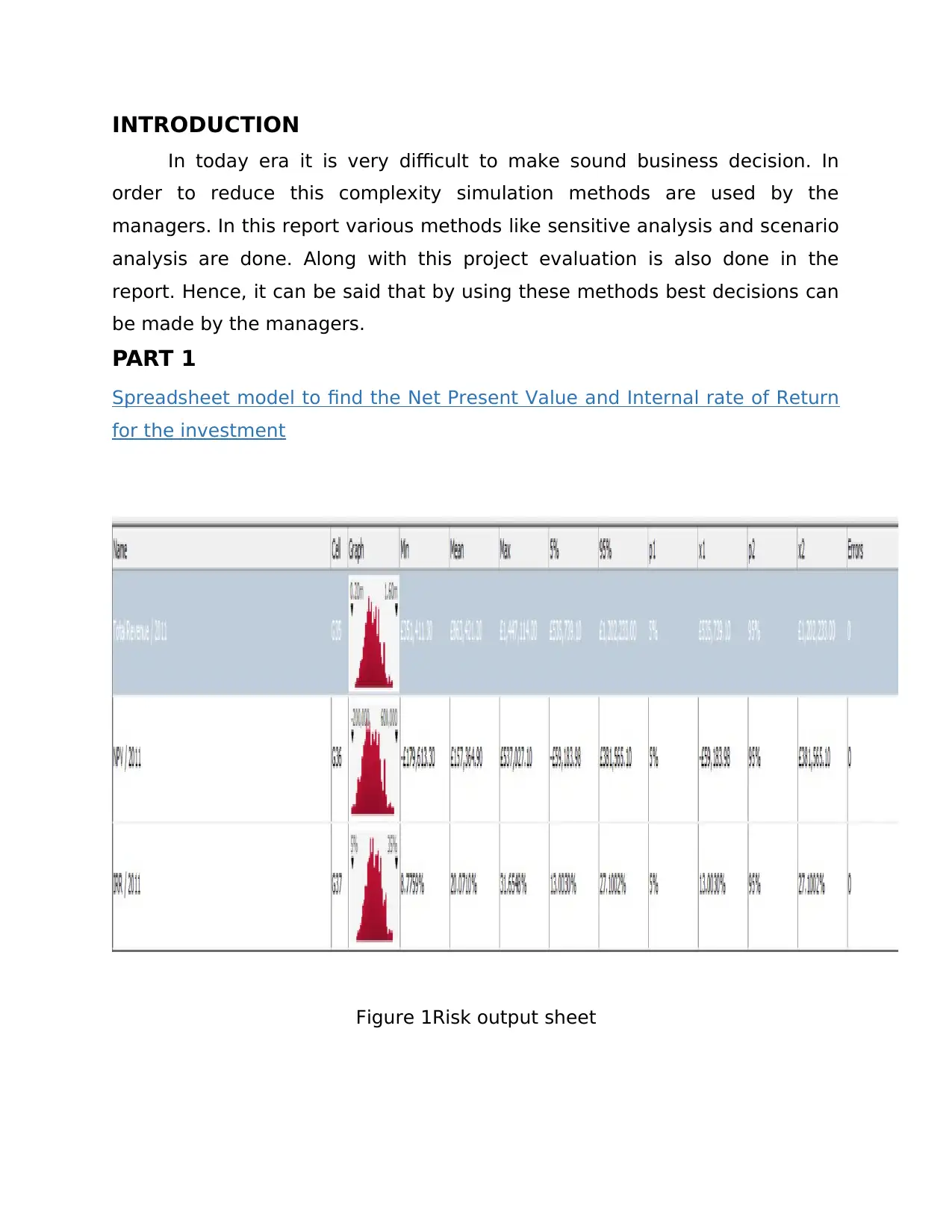
Figure 1Risk output sheet
In today era it is very difficult to make sound business decision. In
order to reduce this complexity simulation methods are used by the
managers. In this report various methods like sensitive analysis and scenario
analysis are done. Along with this project evaluation is also done in the
report. Hence, it can be said that by using these methods best decisions can
be made by the managers.
PART 1
Spreadsheet model to find the Net Present Value and Internal rate of Return
for the investment
Figure 1Risk output sheet
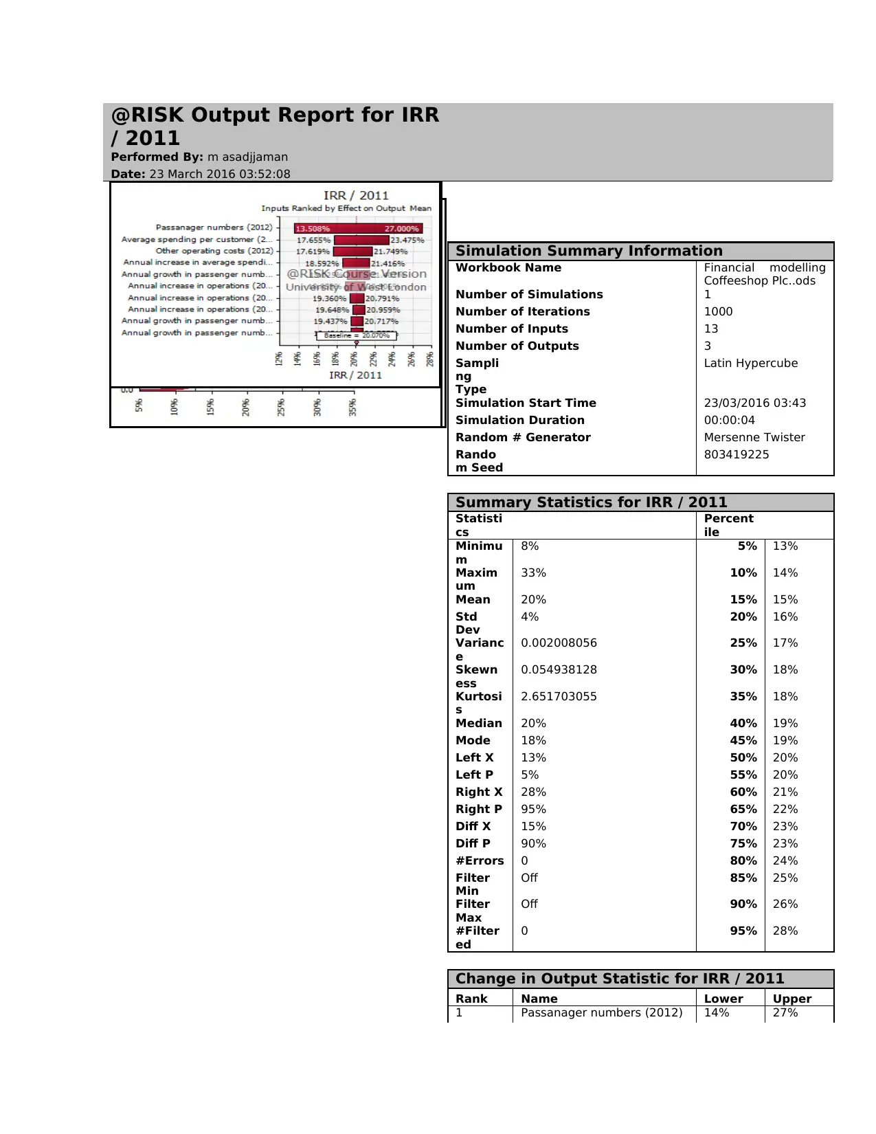
In this attached image results of NPV and IRR are clearly given and helps un
taking decision related to the viability of the project. On the basis of results
produced by the above given table we can see amount that firm may lose in
its business. On the basis of projections financial manager comers to know
about the income that this project can be generate for the firm. The above
given chart shows the maximum, minimum and average return that a firm
can earn on the project during life time of the project. NPV measures the
present value of the project that remain after deducting initial investment
from the present value of the cash flows (Zivot. and Wang, 2007). The cost
of capital for project is 15% which is also discount rate used in the project for
computing present value of the cash flows. On the basis of results produced
by the NPV and IRR best viable can be selected by the firm. Thus, it can be
said that this method help financial managers in selecting most viable
project for the firm. IRR indicate the actual return that a project can earn
on the invested amount. The only difference between ARR and IRR is that in
former method calculation process is tough then latter method of project
evaluation. By using IRR managers can be best decisions related to project
selection. On the basis of analysis of figures given in taqble it can be said
that project is viable for the firm.
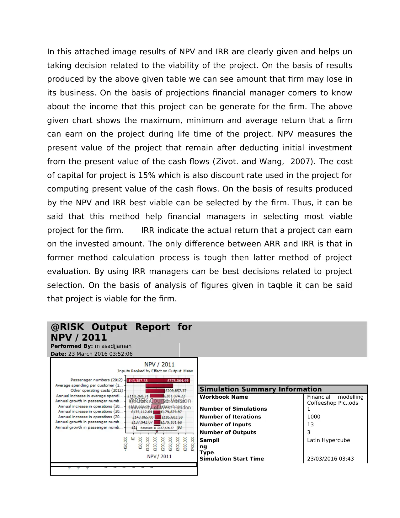
@RISK Output Report for
NPV / 2011
Performed By: m asadjjaman
Date: 23 March 2016 03:52:06
Simulation Summary Information
Workbook Name Financial modelling
Coffeeshop Plc..ods
Number of Simulations 1
Number of Iterations 1000
Number of Inputs 13
Number of Outputs 3
Sampli
ng
Type
Latin Hypercube
Simulation Start Time 23/03/2016 03:43
taking decision related to the viability of the project. On the basis of results
produced by the above given table we can see amount that firm may lose in
its business. On the basis of projections financial manager comers to know
about the income that this project can be generate for the firm. The above
given chart shows the maximum, minimum and average return that a firm
can earn on the project during life time of the project. NPV measures the
present value of the project that remain after deducting initial investment
from the present value of the cash flows (Zivot. and Wang, 2007). The cost
of capital for project is 15% which is also discount rate used in the project for
computing present value of the cash flows. On the basis of results produced
by the NPV and IRR best viable can be selected by the firm. Thus, it can be
said that this method help financial managers in selecting most viable
project for the firm. IRR indicate the actual return that a project can earn
on the invested amount. The only difference between ARR and IRR is that in
former method calculation process is tough then latter method of project
evaluation. By using IRR managers can be best decisions related to project
selection. On the basis of analysis of figures given in taqble it can be said
that project is viable for the firm.
@RISK Output Report for
NPV / 2011
Performed By: m asadjjaman
Date: 23 March 2016 03:52:06
Simulation Summary Information
Workbook Name Financial modelling
Coffeeshop Plc..ods
Number of Simulations 1
Number of Iterations 1000
Number of Inputs 13
Number of Outputs 3
Sampli
ng
Type
Latin Hypercube
Simulation Start Time 23/03/2016 03:43
Secure Best Marks with AI Grader
Need help grading? Try our AI Grader for instant feedback on your assignments.
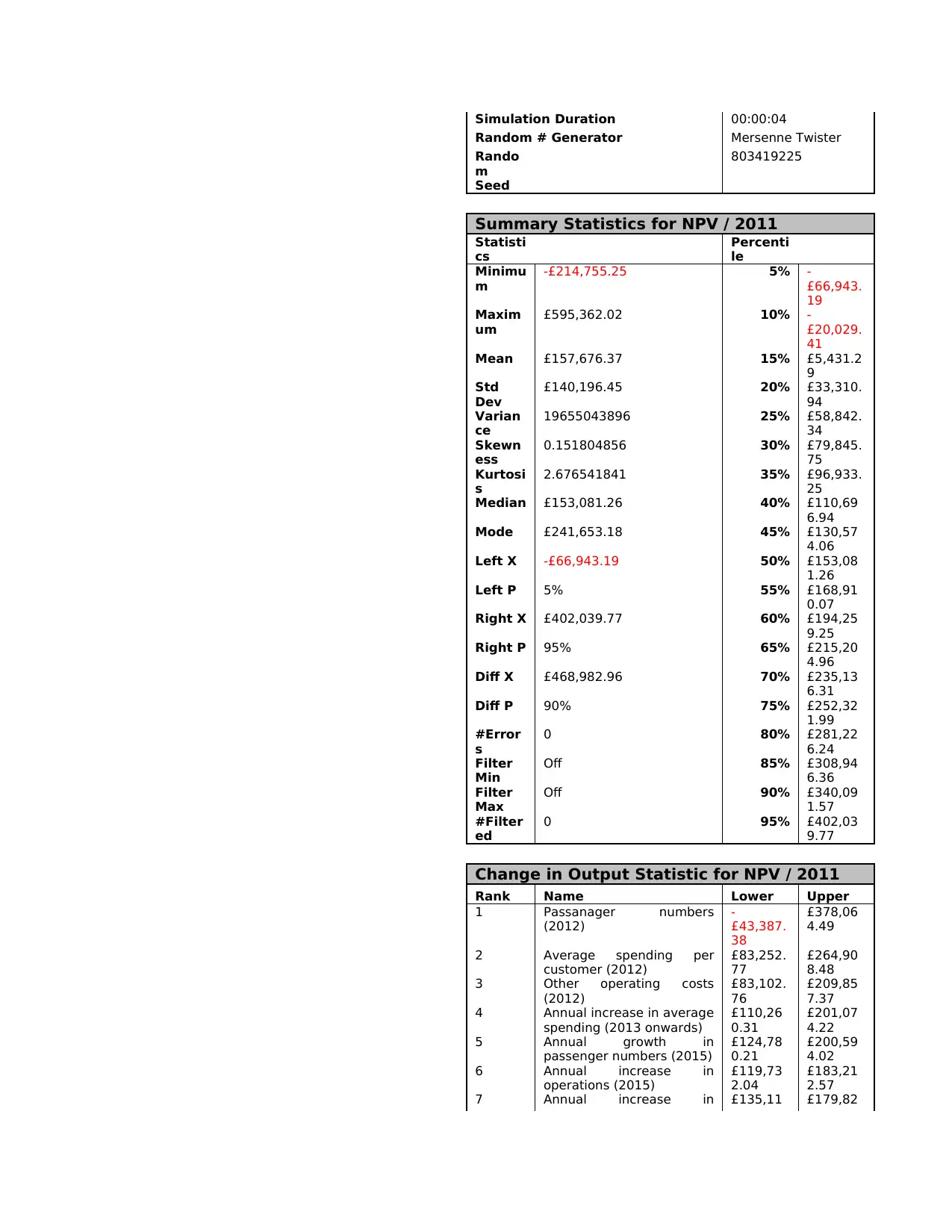
Simulation Duration 00:00:04
Random # Generator Mersenne Twister
Rando
m
Seed
803419225
Summary Statistics for NPV / 2011
Statisti
cs
Percenti
le
Minimu
m
-£214,755.25 5% -
£66,943.
19
Maxim
um
£595,362.02 10% -
£20,029.
41
Mean £157,676.37 15% £5,431.2
9
Std
Dev
£140,196.45 20% £33,310.
94
Varian
ce
19655043896 25% £58,842.
34
Skewn
ess
0.151804856 30% £79,845.
75
Kurtosi
s
2.676541841 35% £96,933.
25
Median £153,081.26 40% £110,69
6.94
Mode £241,653.18 45% £130,57
4.06
Left X -£66,943.19 50% £153,08
1.26
Left P 5% 55% £168,91
0.07
Right X £402,039.77 60% £194,25
9.25
Right P 95% 65% £215,20
4.96
Diff X £468,982.96 70% £235,13
6.31
Diff P 90% 75% £252,32
1.99
#Error
s
0 80% £281,22
6.24
Filter
Min
Off 85% £308,94
6.36
Filter
Max
Off 90% £340,09
1.57
#Filter
ed
0 95% £402,03
9.77
Change in Output Statistic for NPV / 2011
Rank Name Lower Upper
1 Passanager numbers
(2012)
-
£43,387.
38
£378,06
4.49
2 Average spending per
customer (2012)
£83,252.
77
£264,90
8.48
3 Other operating costs
(2012)
£83,102.
76
£209,85
7.37
4 Annual increase in average
spending (2013 onwards)
£110,26
0.31
£201,07
4.22
5 Annual growth in
passenger numbers (2015)
£124,78
0.21
£200,59
4.02
6 Annual increase in
operations (2015)
£119,73
2.04
£183,21
2.57
7 Annual increase in £135,11 £179,82

operations (2016) 2.64 9.97
8 Annual increase in
operations (2013)
£143,86
5.00
£185,60
2.58
9 Annual growth in
passenger numbers (2016)
£137,94
2.07
£179,10
1.68
10 Annual growth in
passenger numbers (2013)
£138,92
2.93
£179,89
9.93
8 Annual increase in
operations (2013)
£143,86
5.00
£185,60
2.58
9 Annual growth in
passenger numbers (2016)
£137,94
2.07
£179,10
1.68
10 Annual growth in
passenger numbers (2013)
£138,92
2.93
£179,89
9.93
@RISK Output Report for IRR
/ 2011
Performed By: m asadjjaman
Date: 23 March 2016 03:52:08
Simulation Summary Information
Workbook Name Financial modelling
Coffeeshop Plc..ods
Number of Simulations 1
Number of Iterations 1000
Number of Inputs 13
Number of Outputs 3
Sampli
ng
Type
Latin Hypercube
Simulation Start Time 23/03/2016 03:43
Simulation Duration 00:00:04
Random # Generator Mersenne Twister
Rando
m Seed
803419225
Summary Statistics for IRR / 2011
Statisti
cs
Percent
ile
Minimu
m
8% 5% 13%
Maxim
um
33% 10% 14%
Mean 20% 15% 15%
Std
Dev
4% 20% 16%
Varianc
e
0.002008056 25% 17%
Skewn
ess
0.054938128 30% 18%
Kurtosi
s
2.651703055 35% 18%
Median 20% 40% 19%
Mode 18% 45% 19%
Left X 13% 50% 20%
Left P 5% 55% 20%
Right X 28% 60% 21%
Right P 95% 65% 22%
Diff X 15% 70% 23%
Diff P 90% 75% 23%
#Errors 0 80% 24%
Filter
Min
Off 85% 25%
Filter
Max
Off 90% 26%
#Filter
ed
0 95% 28%
Change in Output Statistic for IRR / 2011
Rank Name Lower Upper
1 Passanager numbers (2012) 14% 27%
Paraphrase This Document
Need a fresh take? Get an instant paraphrase of this document with our AI Paraphraser
2 Average spending per
customer (2012)
18% 23%
3 Other operating costs (2012) 18% 22%
4 Annual increase in average
spending (2013 onwards)
19% 21%
5 Annual growth in passenger
numbers (2015)
19% 21%
6 Annual increase in
operations (2015)
19% 21%
7 Annual increase in
operations (2016)
19% 21%
8 Annual increase in
operations (2013)
20% 21%
9 Annual growth in passenger
numbers (2016)
19% 21%
10 Annual growth in passenger
numbers (2013)
19% 21%
PART B
Simulation on proposed project
@RISK Sensitivity
Analysis
Performed By: m asadjjaman
Date: 23 March 2016 01:35:25
Ran
k
For
G35
Ce
ll
Name Description Sheet1!
G35
Total
Revenue /
2011
Correlatio
n Coeff.
Sheet1!
G36
NPV /
2011
Correlatio
n Coeff.
Sheet1!
G37
IRR / 2011
Correlatio
n Coeff.
#1 B5 Passanager numbers (2012) RiskTriang(1800000,2000000,2300000) 0.87 0.88 0.88
#2 B1
4
Average spending per
customer (2012) RiskNormal(5,0.1) 0.31 0.30 0.30
#3 B1
9 Other operating costs (2012) RiskTriang(280000,300000,330000) -
0.19
-
0.20
-
0.19
#4 B2
2
Annual increase in operations
(2015) RiskNormal(0,10,RiskCorrmat(NewMatrix2,3)) 0.18 0.18 0.18
#5 B9 Annual growth in passenger
numbers (2016)
RiskTriang(1%,1.5%,3%,RiskCorrmat(NewMatri
x1,4)) 0.13 0.12 0.11
#6 B1
5
Annual increase in average
spending (2013 onwards) RiskUniform(0.1,0.2) 0.12 0.09 0.08
#7 B8 Annual growth in passenger
numbers (2015)
RiskTriang(1%,1.5%,3%,RiskCorrmat(NewMatri
x1,3)) 0.08 0.06 0.06
#8 B2
1
Annual increase in operations
(2014) RiskNormal(0,10,RiskCorrmat(NewMatrix2,2)) 0.06 0.06 0.06
#9 B7 Annual growth in passenger
numbers (2014)
RiskTriang(1%,1.5%,3%,RiskCorrmat(NewMatri
x1,2)) 0.03 0.02 0.01
#1
0
B2
3
Annual increase in operations
(2016) RiskNormal(0,10,RiskCorrmat(NewMatrix2,4)) -
0.03
-
0.03
-
0.04
#1
1
B2
0
Annual increase in operations
(2013) RiskNormal(0,10,RiskCorrmat(NewMatrix2,1)) -
0.00
-
0.00
-
0.00

#1
2 B6 Annual growth in passenger
numbers (2013)
RiskTriang(1%,1.5%,3%,RiskCorrmat(NewMatri
x1,1)) 0.00
-
0.01
-
0.02
- B1
7 Gross margin RiskUniform(64%,66%) n/a n/a n/a
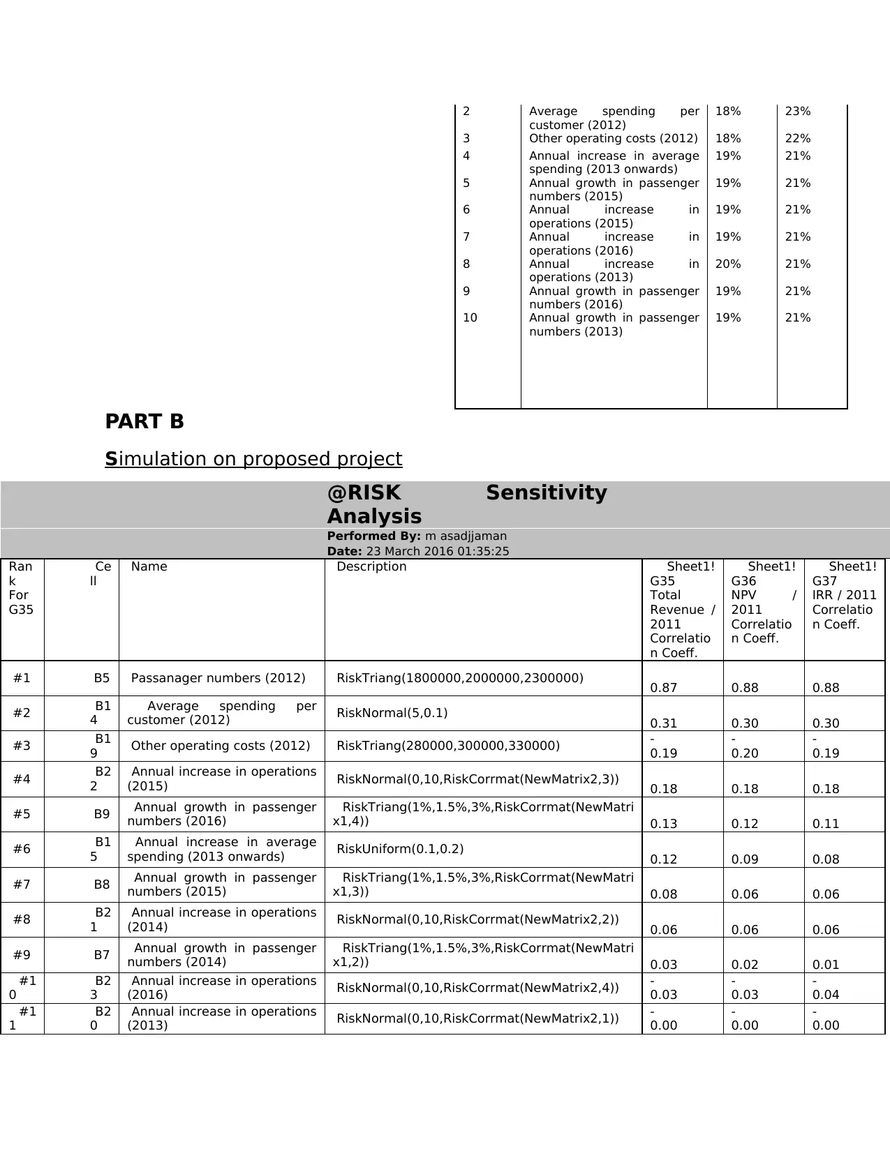
In this image given above sensitive analysis of NPV and IRR is done for entire
project life. In this report different distribution are used like normal
distribution, triangular distribution and uniform distribution. By using same
from different sides project is evaluated. These distributions indicate the
maximum, average and minimum value of the project that is at risk. These
values are shown for each and every type of distribution. Sensitivity analysis
is used to measure changes that can take place in the specific variable with
change in one variable. By looking at the sensitive table manager get an idea
about the likely changes in the value of specific variable due to change in
other variable (Andersen, Bollerslev, T. and Diebold, 2007). The predictions
made by sensitive analysis help managers in making sound business
decisions. This is because there is tolerance level that manager decide
related to the specific variable. Manager will use that tolerance level for in
order to identify the limit up to which he can accept changes in the specific
variable. In the given table values of correlation is given for different factors
and by using values of correlation impact of input on output can be
determined easily. Means that by using value of correlation the extent to
which specific input can affect output is measured in systematic way
(Example models. 2016). Thus, it can be said that along with sensitive
analysis correlation is a important technique that can be used by the
managers in order to identify impact on one variable if other variable value
get changed with passage of time. Hence, it can be said that both sensitive
analysis and correlation have a due importance for the managers.
2 B6 Annual growth in passenger
numbers (2013)
RiskTriang(1%,1.5%,3%,RiskCorrmat(NewMatri
x1,1)) 0.00
-
0.01
-
0.02
- B1
7 Gross margin RiskUniform(64%,66%) n/a n/a n/a
In this image given above sensitive analysis of NPV and IRR is done for entire
project life. In this report different distribution are used like normal
distribution, triangular distribution and uniform distribution. By using same
from different sides project is evaluated. These distributions indicate the
maximum, average and minimum value of the project that is at risk. These
values are shown for each and every type of distribution. Sensitivity analysis
is used to measure changes that can take place in the specific variable with
change in one variable. By looking at the sensitive table manager get an idea
about the likely changes in the value of specific variable due to change in
other variable (Andersen, Bollerslev, T. and Diebold, 2007). The predictions
made by sensitive analysis help managers in making sound business
decisions. This is because there is tolerance level that manager decide
related to the specific variable. Manager will use that tolerance level for in
order to identify the limit up to which he can accept changes in the specific
variable. In the given table values of correlation is given for different factors
and by using values of correlation impact of input on output can be
determined easily. Means that by using value of correlation the extent to
which specific input can affect output is measured in systematic way
(Example models. 2016). Thus, it can be said that along with sensitive
analysis correlation is a important technique that can be used by the
managers in order to identify impact on one variable if other variable value
get changed with passage of time. Hence, it can be said that both sensitive
analysis and correlation have a due importance for the managers.
@RISK Input
Results
Performed By: m asadjjaman
Date: 23 March 2016 02:23:00
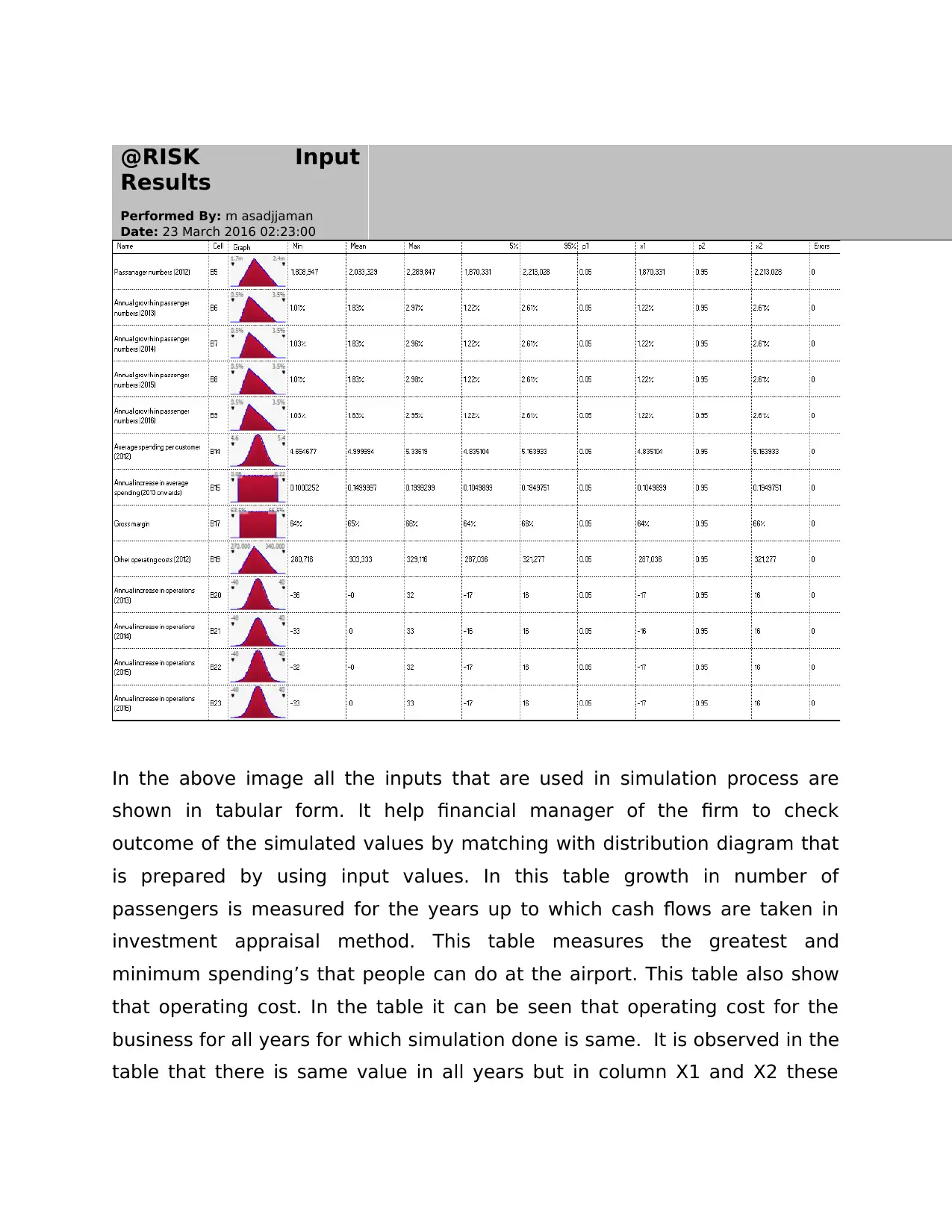
In the above image all the inputs that are used in simulation process are
shown in tabular form. It help financial manager of the firm to check
outcome of the simulated values by matching with distribution diagram that
is prepared by using input values. In this table growth in number of
passengers is measured for the years up to which cash flows are taken in
investment appraisal method. This table measures the greatest and
minimum spending’s that people can do at the airport. This table also show
that operating cost. In the table it can be seen that operating cost for the
business for all years for which simulation done is same. It is observed in the
table that there is same value in all years but in column X1 and X2 these
Results
Performed By: m asadjjaman
Date: 23 March 2016 02:23:00
In the above image all the inputs that are used in simulation process are
shown in tabular form. It help financial manager of the firm to check
outcome of the simulated values by matching with distribution diagram that
is prepared by using input values. In this table growth in number of
passengers is measured for the years up to which cash flows are taken in
investment appraisal method. This table measures the greatest and
minimum spending’s that people can do at the airport. This table also show
that operating cost. In the table it can be seen that operating cost for the
business for all years for which simulation done is same. It is observed in the
table that there is same value in all years but in column X1 and X2 these
Secure Best Marks with AI Grader
Need help grading? Try our AI Grader for instant feedback on your assignments.
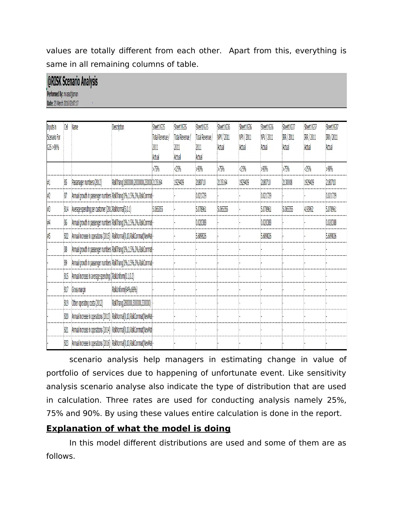
values are totally different from each other. Apart from this, everything is
same in all remaining columns of table.
scenario analysis help managers in estimating change in value of
portfolio of services due to happening of unfortunate event. Like sensitivity
analysis scenario analyse also indicate the type of distribution that are used
in calculation. Three rates are used for conducting analysis namely 25%,
75% and 90%. By using these values entire calculation is done in the report.
Explanation of what the model is doing
In this model different distributions are used and some of them are as
follows.
Probability distribution- It helps in measuring uncertainty in the all
variables of the risk analysis (Bielecki. and Rutkowski, 2013).
Normal distribution- it indicate the mean value of the variable and
standard deviation in the variable value from mean.
Uniform distribution- It indicate the values that have equal chance
of occurrence.
Model limitations
The main limitation of this model is that everyone can not apply this
model. Only person that have good knowledge can apply this model
(Wilmott, 2013). Hence, it can be said that this technique is very complex
and it is its main limitation.
CONCLUSION
On the basis of above discussion it is concluded that managers must
different financial modeling techniques in order to select most viable project
for the business. By using these methods various aspects of project can be
measured and good decision can be taken by the manager.
REFRENCES
Books & journals
Andersen, T.G., Bollerslev, T. and Diebold, F.X., 2007. Roughing it up:
Including jump components in the measurement, modeling, and
forecasting of return volatility. The review of economics and statistics.
89(4). pp.701-720.
Bielecki, T.R. and Rutkowski, M., 2013. Credit risk: modeling, valuation and
hedging. Springer Science & Business Media.
Wilmott, P., 2013. Paul Wilmott on quantitative finance. John Wiley & Sons.
Zivot, E. and Wang, J., 2007. Modeling financial time series with S-Plus® (Vol.
191). Springer Science & Business Media.
Online
Example models. 2016. [Online]. Available through: <
http://www.palisade.com/models/finance.asp>. [Accessed on 23rd March
2016].
1 out of 13
Related Documents


Your All-in-One AI-Powered Toolkit for Academic Success.
+13062052269
info@desklib.com
Available 24*7 on WhatsApp / Email
![[object Object]](/_next/static/media/star-bottom.7253800d.svg)
Unlock your academic potential
© 2024 | Zucol Services PVT LTD | All rights reserved.