BE314 Financial Modeling Report: Coffee Export Analysis, Singapore
VerifiedAdded on 2022/08/25
|7
|1052
|22
Report
AI Summary
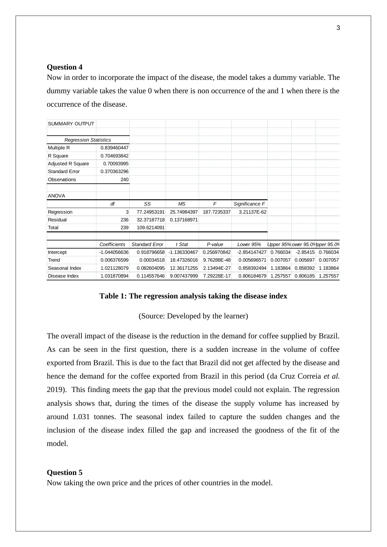
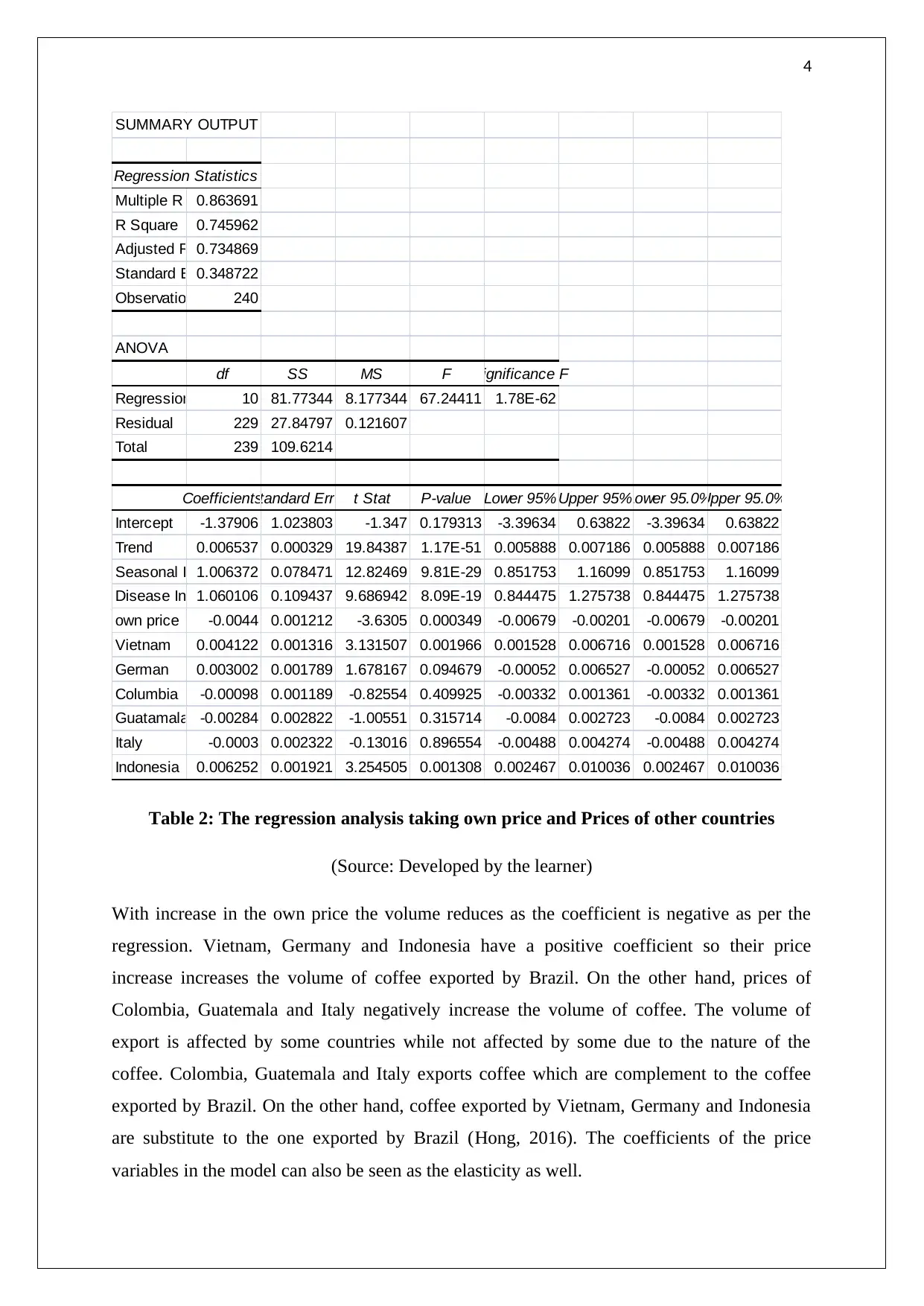
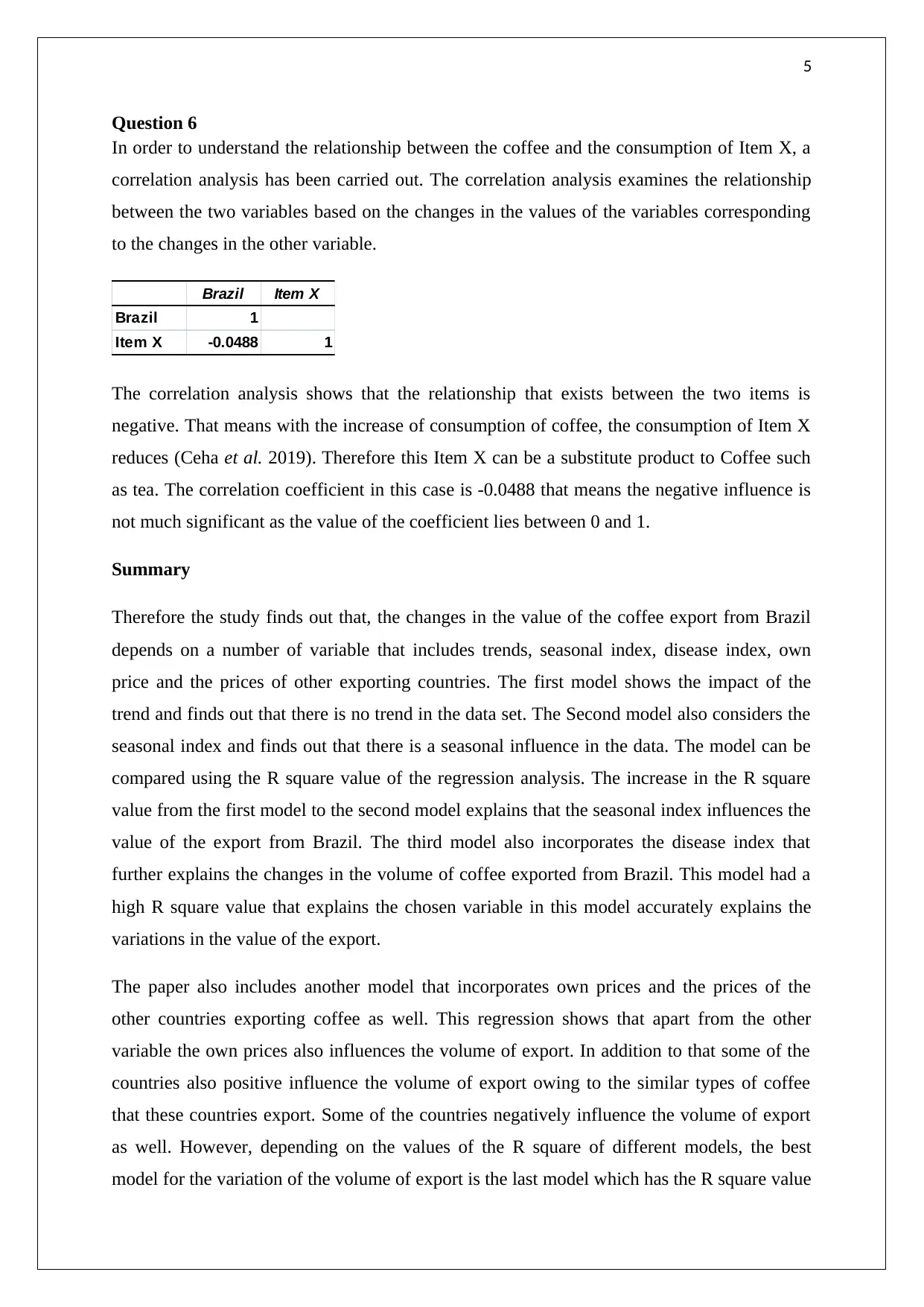
This report analyzes the financial modeling of coffee exports, focusing on data from Brazil. The analysis employs regression techniques to examine the impact of various factors on export volume, including trends, seasonal indices, and disease outbreaks. The study incorporates dummy variables to assess the influence of diseases and considers both the own price and the prices of competing countries. Correlation analysis is used to explore the relationship between coffee consumption and the consumption of a substitute product. The findings reveal the significance of factors like seasonal indices, disease, and prices in influencing coffee export volumes. The best model, with an R-squared value of 0.74, highlights the combined influence of seasonal indices, disease, own price, and the prices of other countries. The report concludes that understanding these variables is crucial for predicting and managing coffee export volumes.
1 out of 7

Your All-in-One AI-Powered Toolkit for Academic Success.
+13062052269
info@desklib.com
Available 24*7 on WhatsApp / Email
![[object Object]](/_next/static/media/star-bottom.7253800d.svg)
Copyright © 2020–2025 A2Z Services. All Rights Reserved. Developed and managed by ZUCOL.