Finite Element Modelling of Stiffened Plate: Abaqus Analysis
VerifiedAdded on 2020/05/28
|15
|1164
|75
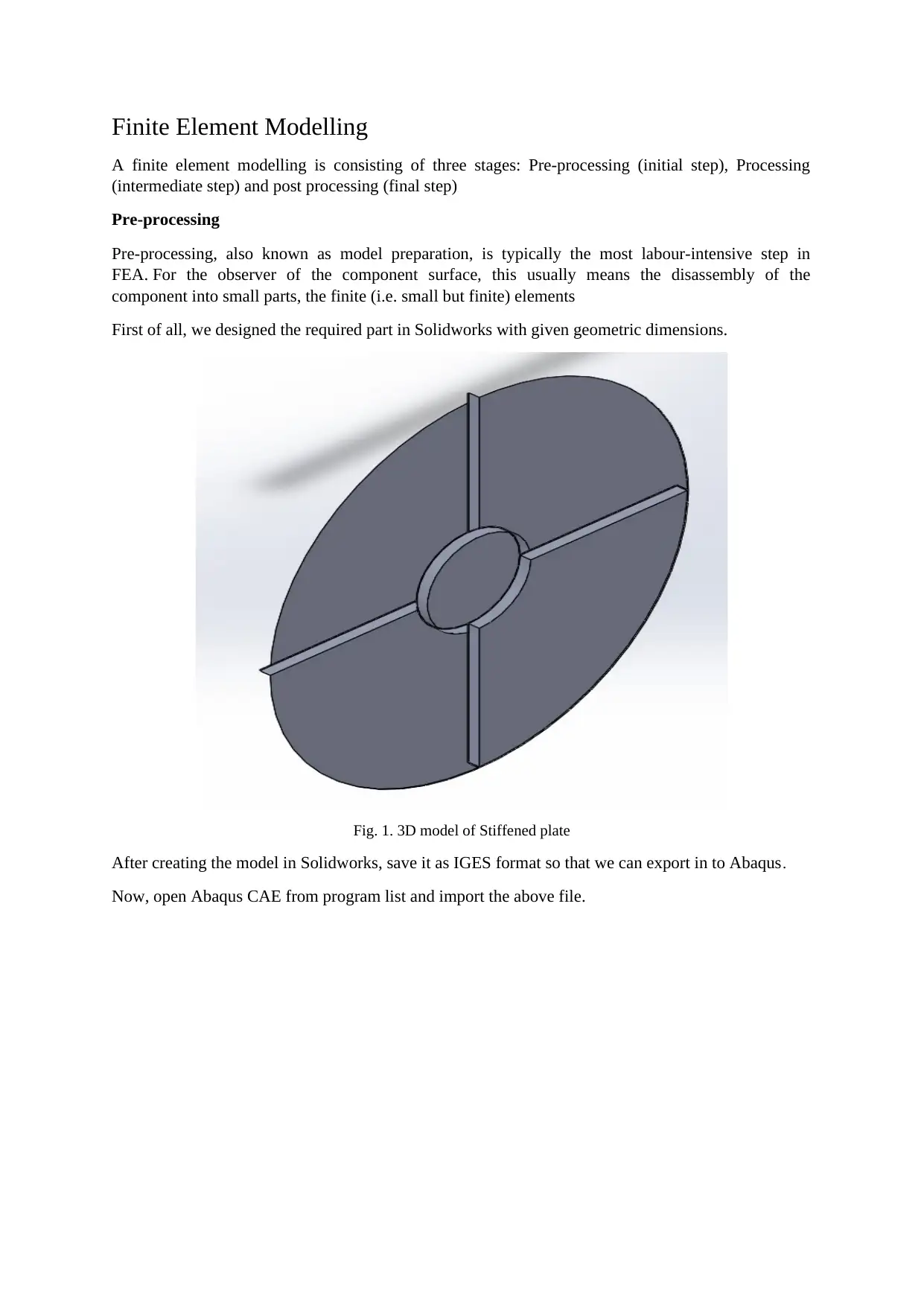
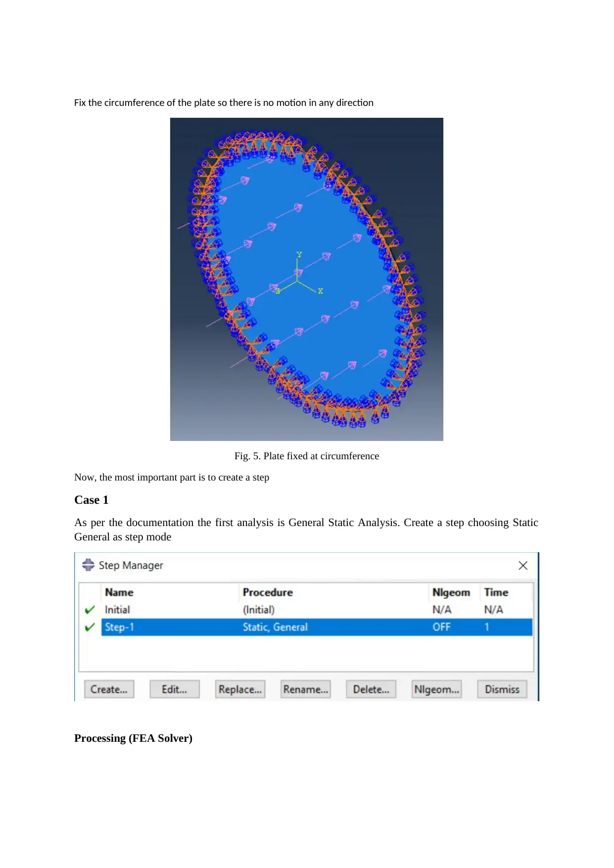
Practical Assignment
AI Summary
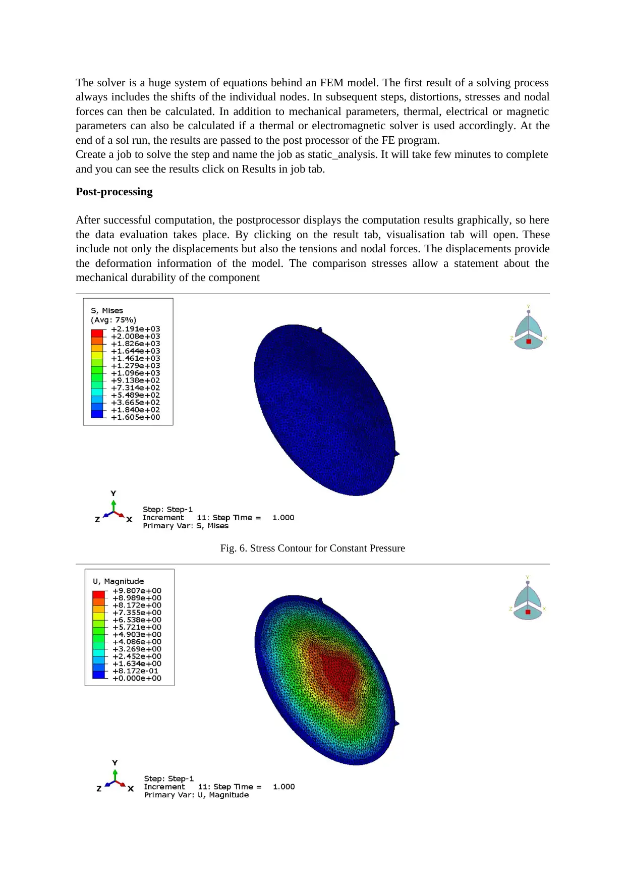
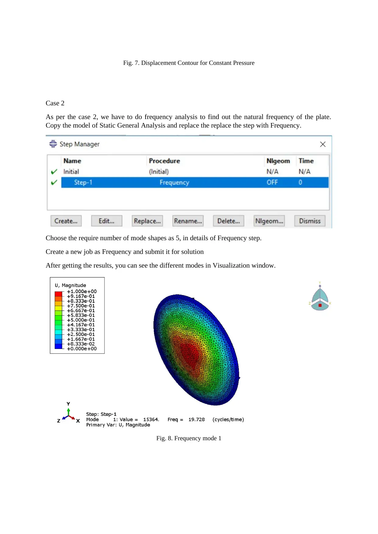
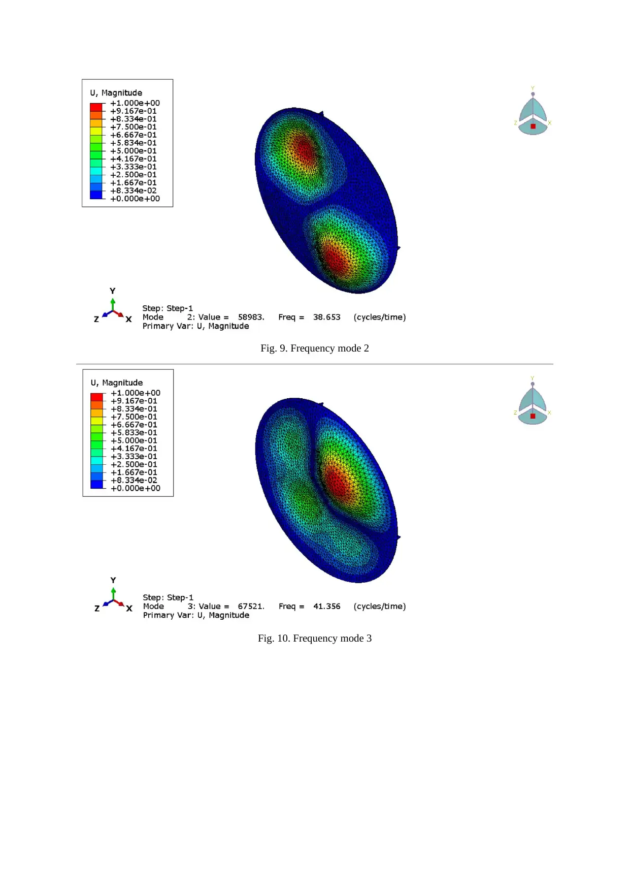
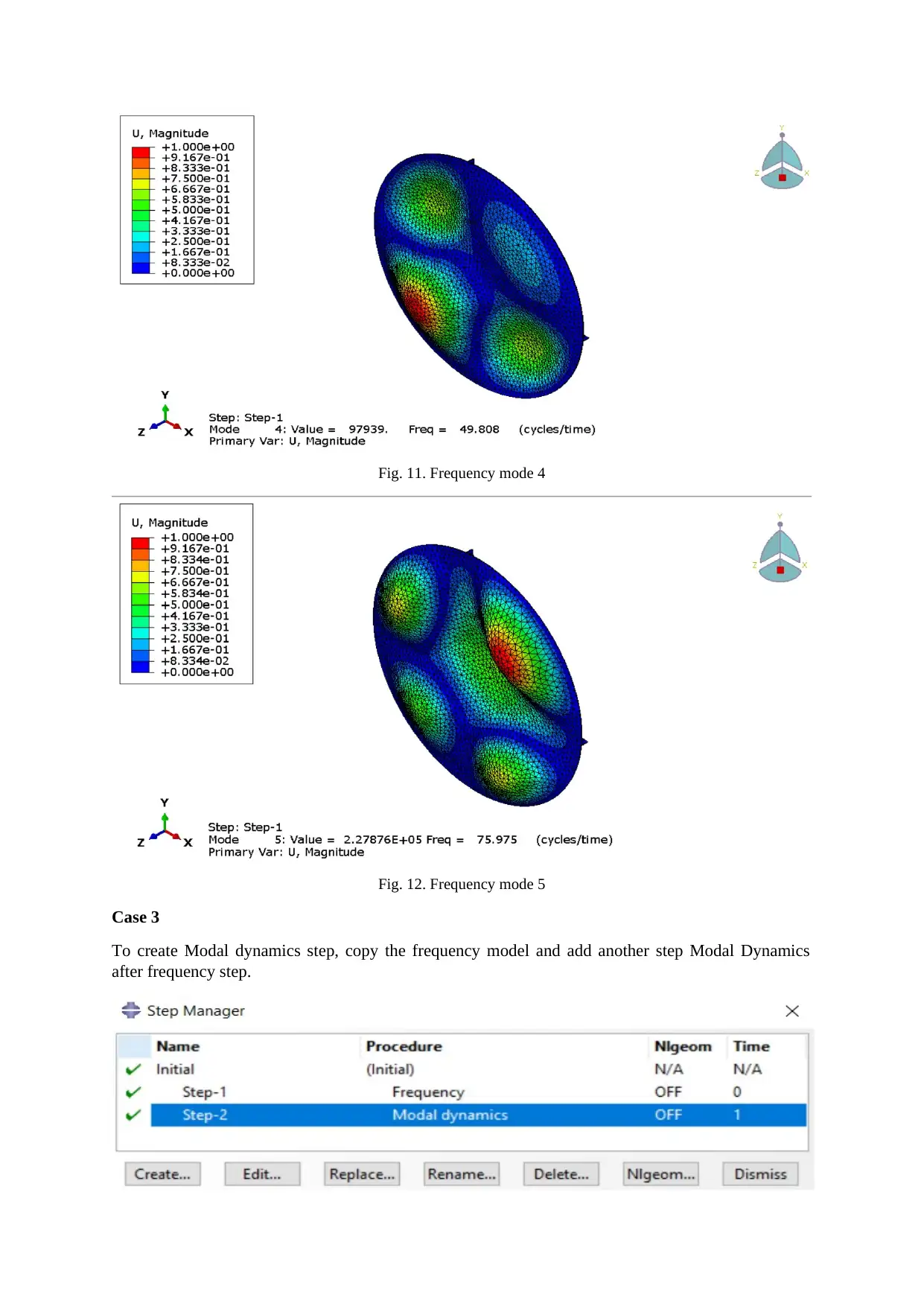
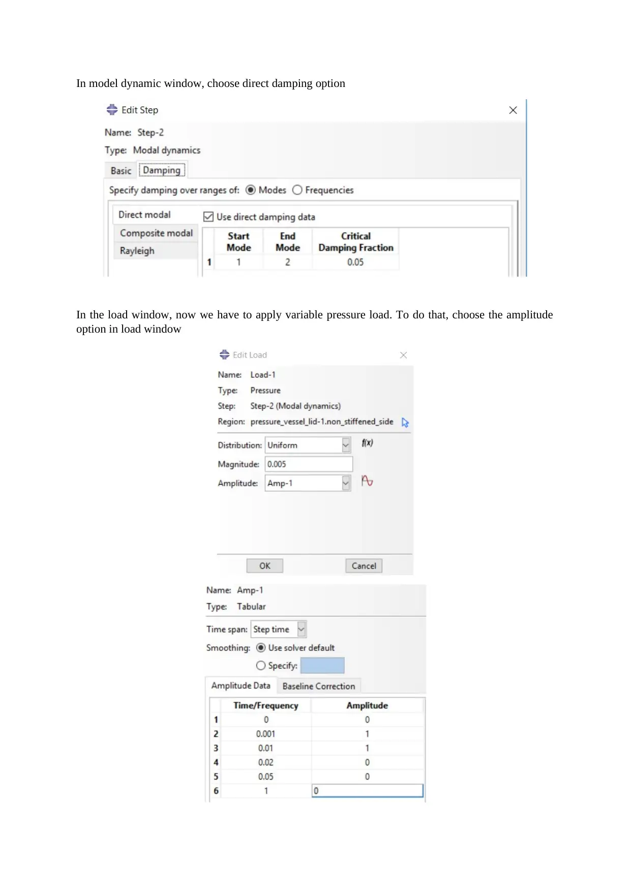
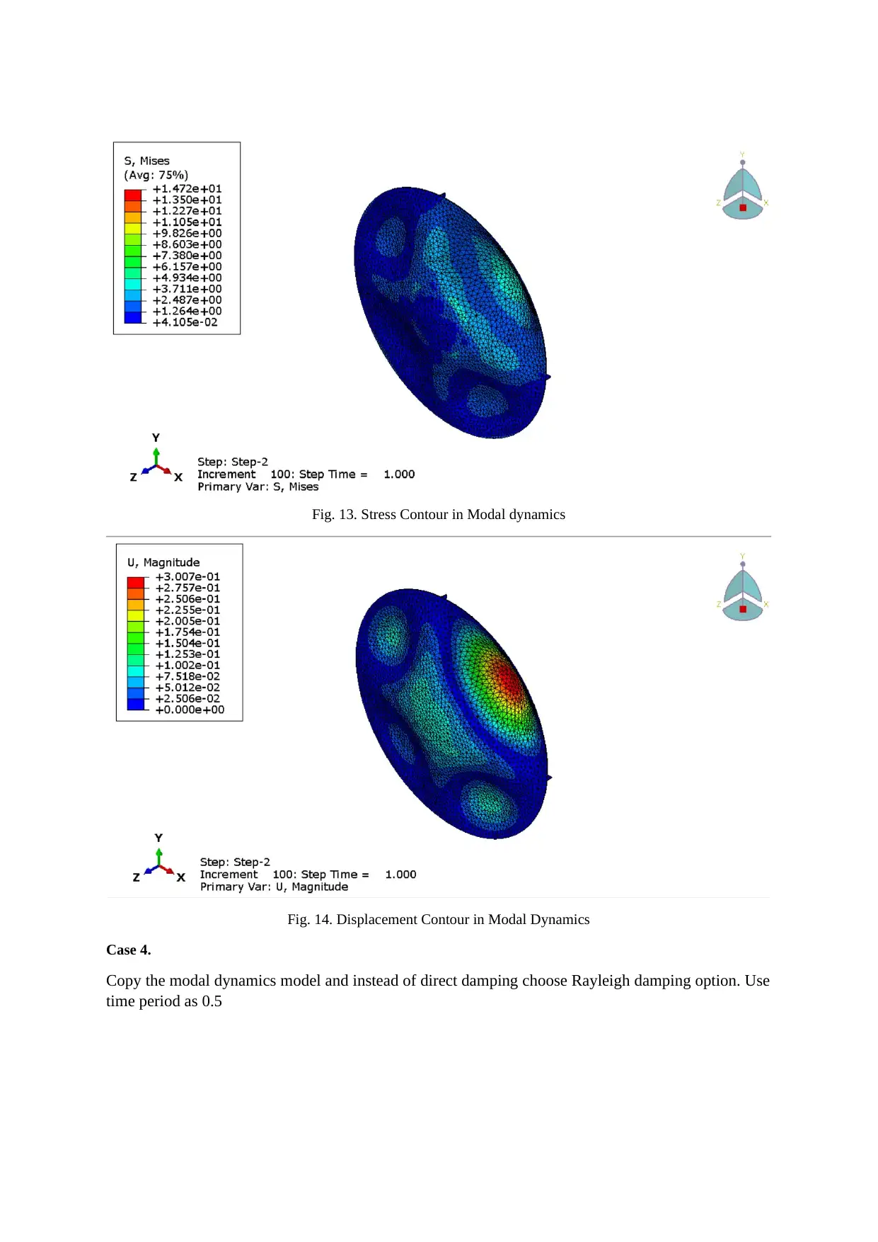
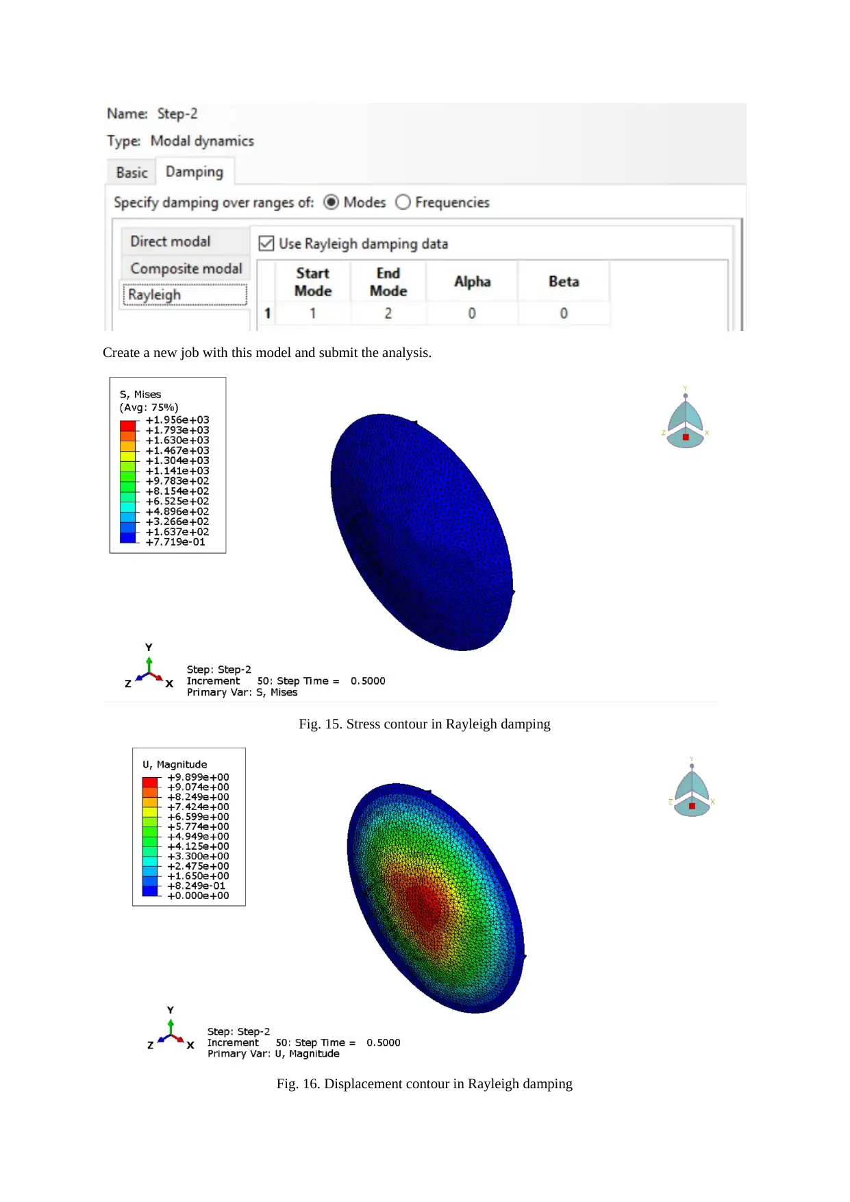
This assignment details a finite element modeling (FEM) analysis of a stiffened plate using Abaqus software. The solution progresses through three stages: pre-processing, processing, and post-processing. Pre-processing involves creating a 3D model in Solidworks and importing it into Abaqus, assigning material properties (steel), and meshing the geometry. Boundary conditions and loads, including pressure, are applied. The processing stage involves running various analyses, including static general analysis, frequency analysis to determine natural frequencies, and modal dynamics with both direct and Rayleigh damping. The assignment also covers explicit dynamics analysis with changes in material properties. Post-processing involves visualizing and interpreting results such as stress and displacement contours for each case.
1 out of 15
Related Documents


Your All-in-One AI-Powered Toolkit for Academic Success.
+13062052269
info@desklib.com
Available 24*7 on WhatsApp / Email
![[object Object]](/_next/static/media/star-bottom.7253800d.svg)
Copyright © 2020–2026 A2Z Services. All Rights Reserved. Developed and managed by ZUCOL.