Operations Research: Flow Networks and Inventory Control

This operations research assignment explores concepts of flow networks and inventory control. It involves analyzing a production network with multiple components and determining the maximum flow through it. The assignment also delves into economic order quantity (EOQ) calculation, considering ordering costs, holding costs, and demand to find the optimal order size for inventory management.

Monash University
Faculty of Information Technology
FIT5097 Business Intelligence Modelling
2nd Semester 2017

Table of Contents
Problem 1:........................................................................................................................................3
Part A:..........................................................................................................................................3
Part d:...........................................................................................................................................4
Part e:...........................................................................................................................................4
Part f:...........................................................................................................................................4
Part g:...........................................................................................................................................4
Part h:...........................................................................................................................................4
Part i:............................................................................................................................................5
Part j:............................................................................................................................................5
Part k:...........................................................................................................................................5
Part l:............................................................................................................................................6
Part m:..........................................................................................................................................6
Part o:...........................................................................................................................................6
Problem 2:........................................................................................................................................6
Part A:..........................................................................................................................................6
Part c:...........................................................................................................................................7
Part d:...........................................................................................................................................7
Part f:...........................................................................................................................................8
Part g:...........................................................................................................................................8
Part h:...........................................................................................................................................8
Part i:............................................................................................................................................8
Part j:............................................................................................................................................9
Part k:...........................................................................................................................................9
Problem 3:........................................................................................................................................9

Problem 1:
Part A:
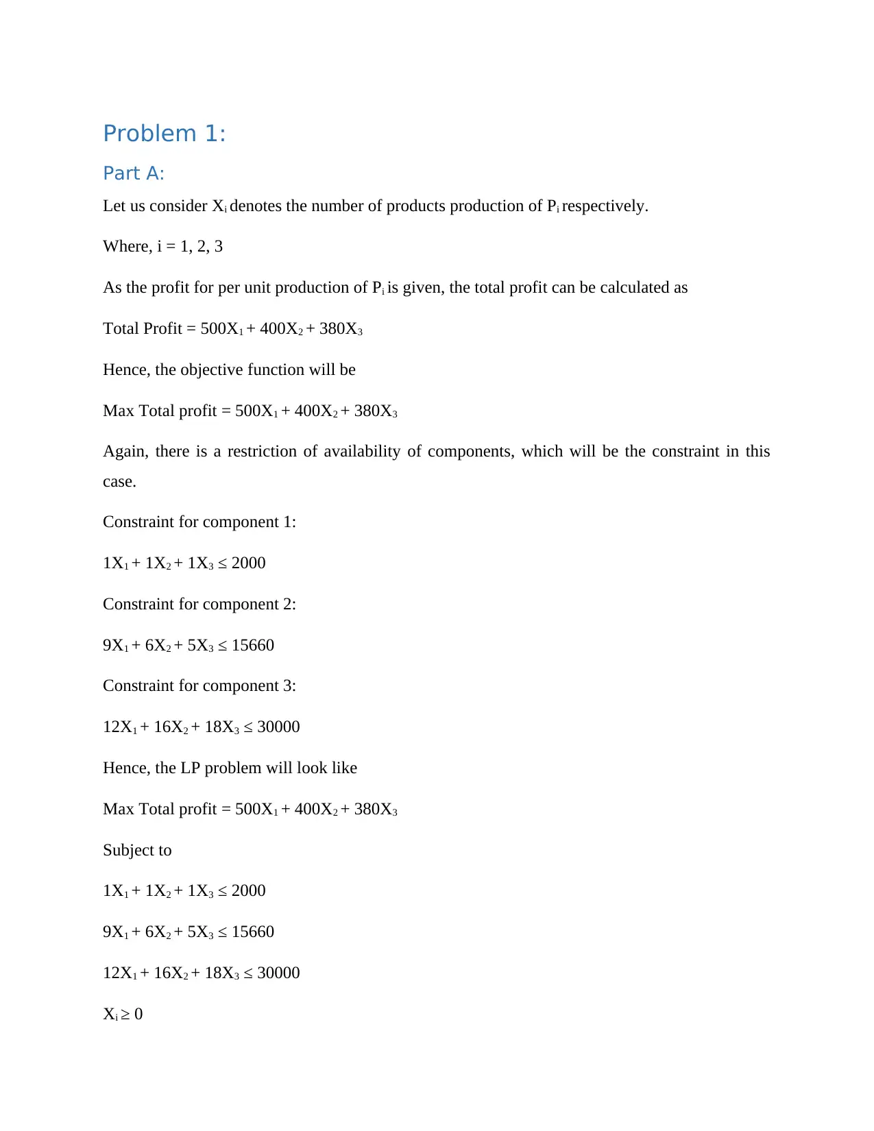
Let us consider Xi denotes the number of products production of Pi respectively.
Where, i = 1, 2, 3
As the profit for per unit production of Pi is given, the total profit can be calculated as
Total Profit = 500X1 + 400X2 + 380X3
Hence, the objective function will be
Max Total profit = 500X1 + 400X2 + 380X3
Again, there is a restriction of availability of components, which will be the constraint in this
case.
Constraint for component 1:
1X1 + 1X2 + 1X3 ≤ 2000
Constraint for component 2:
9X1 + 6X2 + 5X3 ≤ 15660
Constraint for component 3:
12X1 + 16X2 + 18X3 ≤ 30000
Hence, the LP problem will look like
Max Total profit = 500X1 + 400X2 + 380X3
Subject to
1X1 + 1X2 + 1X3 ≤ 2000
9X1 + 6X2 + 5X3 ≤ 15660
12X1 + 16X2 + 18X3 ≤ 30000
Xi ≥ 0

Part d:
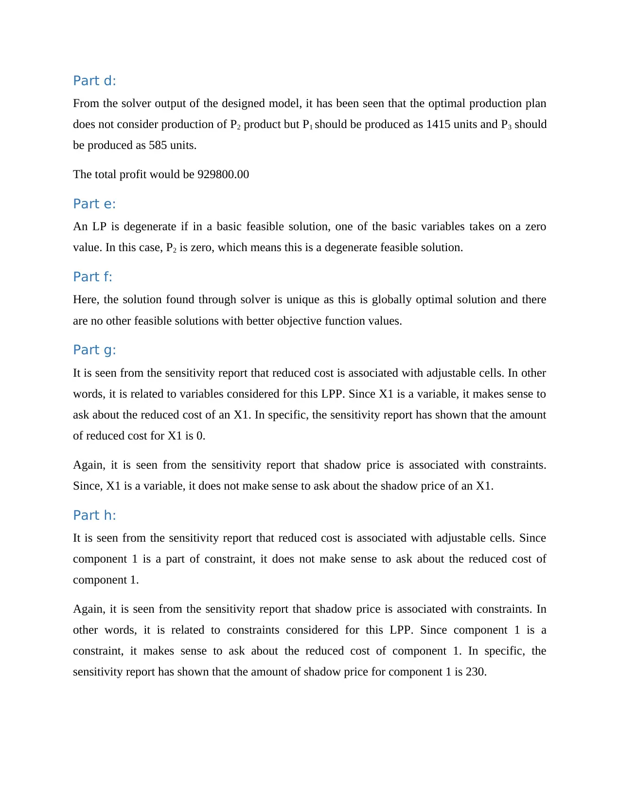
From the solver output of the designed model, it has been seen that the optimal production plan
does not consider production of P2 product but P1 should be produced as 1415 units and P3 should
be produced as 585 units.
The total profit would be 929800.00
Part e:
An LP is degenerate if in a basic feasible solution, one of the basic variables takes on a zero
value. In this case, P2 is zero, which means this is a degenerate feasible solution.
Part f:
Here, the solution found through solver is unique as this is globally optimal solution and there
are no other feasible solutions with better objective function values.
Part g:
It is seen from the sensitivity report that reduced cost is associated with adjustable cells. In other
words, it is related to variables considered for this LPP. Since X1 is a variable, it makes sense to
ask about the reduced cost of an X1. In specific, the sensitivity report has shown that the amount
of reduced cost for X1 is 0.
Again, it is seen from the sensitivity report that shadow price is associated with constraints.
Since, X1 is a variable, it does not make sense to ask about the shadow price of an X1.
Part h:
It is seen from the sensitivity report that reduced cost is associated with adjustable cells. Since
component 1 is a part of constraint, it does not make sense to ask about the reduced cost of
component 1.
Again, it is seen from the sensitivity report that shadow price is associated with constraints. In
other words, it is related to constraints considered for this LPP. Since component 1 is a
constraint, it makes sense to ask about the reduced cost of component 1. In specific, the
sensitivity report has shown that the amount of shadow price for component 1 is 230.

Part i:
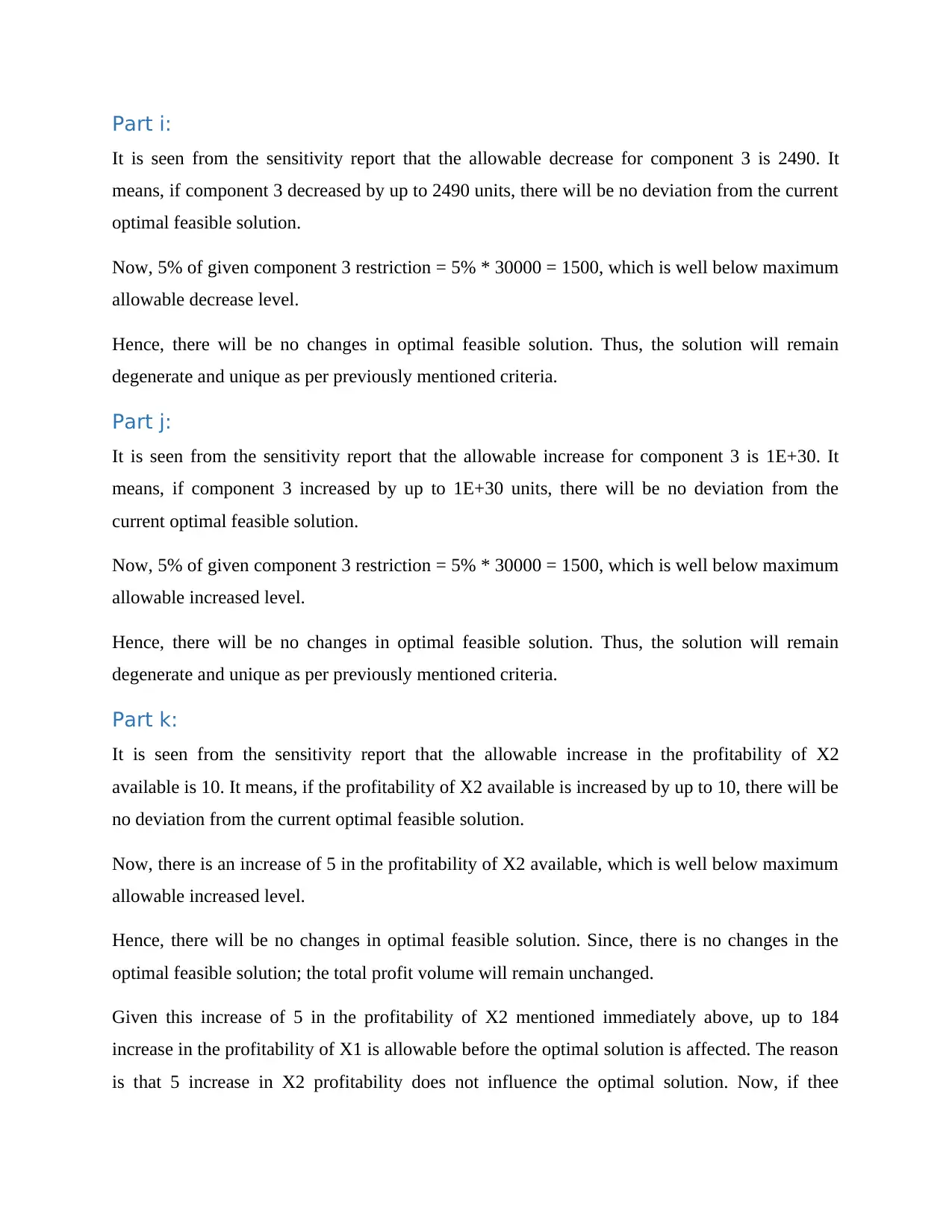
It is seen from the sensitivity report that the allowable decrease for component 3 is 2490. It
means, if component 3 decreased by up to 2490 units, there will be no deviation from the current
optimal feasible solution.
Now, 5% of given component 3 restriction = 5% * 30000 = 1500, which is well below maximum
allowable decrease level.
Hence, there will be no changes in optimal feasible solution. Thus, the solution will remain
degenerate and unique as per previously mentioned criteria.
Part j:
It is seen from the sensitivity report that the allowable increase for component 3 is 1E+30. It
means, if component 3 increased by up to 1E+30 units, there will be no deviation from the
current optimal feasible solution.
Now, 5% of given component 3 restriction = 5% * 30000 = 1500, which is well below maximum
allowable increased level.
Hence, there will be no changes in optimal feasible solution. Thus, the solution will remain
degenerate and unique as per previously mentioned criteria.
Part k:
It is seen from the sensitivity report that the allowable increase in the profitability of X2
available is 10. It means, if the profitability of X2 available is increased by up to 10, there will be
no deviation from the current optimal feasible solution.
Now, there is an increase of 5 in the profitability of X2 available, which is well below maximum
allowable increased level.
Hence, there will be no changes in optimal feasible solution. Since, there is no changes in the
optimal feasible solution; the total profit volume will remain unchanged.
Given this increase of 5 in the profitability of X2 mentioned immediately above, up to 184
increase in the profitability of X1 is allowable before the optimal solution is affected. The reason
is that 5 increase in X2 profitability does not influence the optimal solution. Now, if thee

sensitivity report is taken into consideration, then it can be found that maximum allowable
restriction is 184. Hence, up to that limit there will be no deviation from current profit level.
Part l:
Suppose that we want to make a new product, P4, requiring 1 of Component1, 2 of Component2,
3 of Component3; and P4 sells at a profit of $250. We should make any of P4 as there will be no
changes in the optimal feasible solution.
At least $40 more profitable would P4 have to be before we would make it.
Part m:
As Xi is considered as integer; the non negativity constraints needs to be changed in excel solver.
Even though, non negative constraints changed to integer; there would be no changes in optimal
solution.
Part o:
In this case, there would be three additional constraints as X1<=1200; X2<=1200; and
X3<=1200
After adding all three constraints in the above model, it has found that the optimal solution will
look like: P1 = 1200; P2 = 800; P3 = 0; and total profit would be 920000 for both integer and
non-integer value of Xi.
Problem 2:
Part A:
Suppose we are given travelling time tij associated with edge (or directed arc) (i,j). Designate
one node o(origin) as a source node or node from where goods are to be transported and another
node as d or destination node where the goods will finally land up.
To formulate this problem as LPP, we introduce a variable xij as follows
xij= {1 ,∧edge (i, j)is a part of the path
0 , if otherwise
So, xij ∈ {0, 1}, ∀(i, j) ∈ E is a binary variable. The path with shortest travel time can be found
by considering the starting with capacity bo = 1 and destination node with capacity bd = −1

(recipient). All other nodes in between the network are considered as only transshipment nodes
(so bj = 0) with nothing originated from it and nothing is consumed at them. The LPP model is
then as follows:
Min ∑
i
j
tij xij
Subject to
∑
k /( j , k)
x jk − ∑
i /(i , j)
xij=b j
0<= xij <= 1
And bj = {1 if j =0; -1 if j = d; j = 0 for other value of j}
Part c:
From the excel solver solution, it has seen that the minimum cost is 1500.
Part d:
Consider a network two distinguished nodes o and d (respectively, the source node and the
sink/destination node). Each arc has an associated capacity uij but no associated cost. We assume
that there is no edge from d to o. In a max-flow problem, the goal is to maximize the total flow
from o to d.
The numerals along the arcs are the uij values (or arc capacity). The problem is to find maximum
flow that can be send from o ot d.
To formulate this problem as a LPP we introduce an auxiliary edge (d,o) with unlimited capacity
and aim to maximize flwo across this arc. The max-flow problem then can be written as follows
Max xdo
Subject to
∑
k /( j , k)
x jk − ∑
i /(i , j)
xij=0
0<= xij <= uij

Part f:
From the excel solver solution, it can be said that the maximal flow is 25000.
Part g:
It is possible to improve the solution found in part f. in order to do this, following changes
required in excel solver:
Objective function:
Max xdo + 0.01(500X1 + 400X2 + 380X3)
Additional constraints:
Flow of HS + 2000 <= 120000
Flow of JS + 15660 <= 110000
Flow of KS + 30000 <= 110000
In addition, there are two more constraints as mentioned below:
Constraint for component 2:
9X1 + 6X2 + 5X3 ≤ 15660
Constraint for component 3:
12X1 + 16X2 + 18X3 ≤ 30000
Using this revised LPP, the maximum flow become = 259523 appx.
This indicates that there is an improvement of 9523 units of flow.
Part h:
Not counting the edge SA, 10 edges have non-zero flow.
Part i:
In both cases the minimum number is 8.

Part j:
If we allow 1 less edges than above, there will be a reduction of 10000 flow from maximum
flow. Hence new maximum flow will be 250000-10000 = 240000
Part k:
Part 1: total cost = total cost of edges – total cost of edges with 0 flow
= 12600 – 5700 = 690
Part 2: total cost = the cost of that edge * the volume of flow along that edge
= 530000000
Problem 3:
Data Results
d = 5000 (demand/year)
K = $15 (oder cost) Additional cost $20.70
h = $0.10 (unit holding cost) Annual ordering Cost $72.46
c0 0.02 Q<=4150 Annual Holding Cost $51.75
c1 0.0195 Q>4150 Total Variable Cost $144.91
Decision
Optimal
EOQ =
1035
And Economic order quantity (Q*) = square root of [(2 x demand x ordering costs) ÷ holding
costs]
= sqrt(2*5000*15/0.10)
= 1225