Fixed Income Securities and Interest Rate Modelling | Assignment

Fixed Income Securities and Interest Rate Modelling 1
FIXED INCOME SECURITIES AND INTEREST RATE MODELLING
by Student’s Name
Code + Course Name
Professor’s Name
University Name
City, State
Date

Fixed Income Securities and Interest Rate Modelling 2
Fixed Income Securities and Interest Rate Modelling
1.
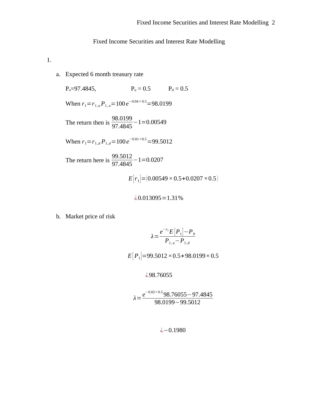
a. Expected 6 month treasury rate
Po=97.4845, Pu = 0.5 Pd = 0.5
When r1=r1 ,u P1 , u=100 e−0.04 × 0.5=98.0199
The return then is 98.0199
97.4845 −1=0.00549
When r1=r1 ,d P1 ,d =100 e−0.01 ×0.5 =99.5012
The return here is 99.5012
97.4845 −1=0.0207
E [ r1 ]= ( 0.00549 × 0.5+0.0207 ×0.5 )
¿ 0.013095=1.31%
b. Market price of risk
λ= e−r0
E [ P1 ] −P0
P1 , u−P1 ,d
E [ P1 ]=99.5012 ×0.5+98.0199× 0.5
¿ 98.76055
λ= e−0.02× 0.5 98.76055−97.4845
98.0199−99.5012
¿−0.1980

Fixed Income Securities and Interest Rate Modelling 3
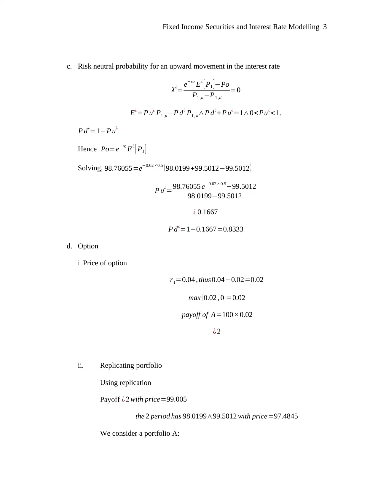
c. Risk neutral probability for an upward movement in the interest rate
λ¿= e−ro E¿ [ P1 ]−Po
P1 ,u −P1 ,d
=0
E¿=P u¿ P1 ,u−P d¿ P1 , d∧P d¿+P u¿=1∧0<Pu¿<1 ,
P d¿=1−P u¿
Hence Po=e−ro E¿ [ P1 ]
Solving, 98.76055=e−0.02 ×0.5 ( 98.0199+99.5012−99.5012 )
P u¿=98.76055 e−0.02 × 0.5−99.5012
98.0199−99.5012
¿ 0.1667
P d¿=1−0.1667=0.8333
d. Option
i. Price of option
r1=0.04 , thus0.04−0.02=0.02
max {0.02 , 0 }=0.02
payoff of A=100× 0.02
¿ 2
ii. Replicating portfolio
Using replication
Payoff ¿ 2 with price=99.005
the 2 period has 98.0199∧99.5012 with price=97.4845
We consider a portfolio A:

Fixed Income Securities and Interest Rate Modelling 4
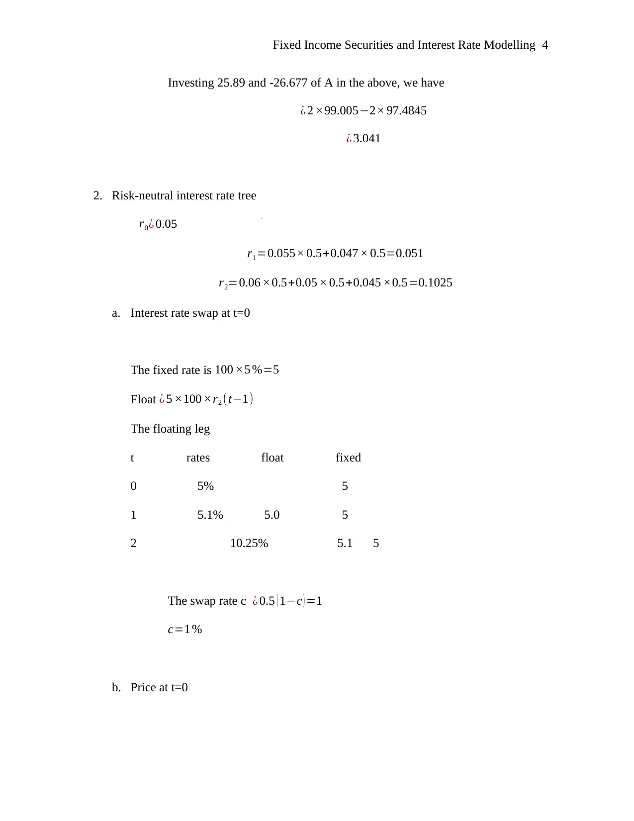
Investing 25.89 and -26.677 of A in the above, we have
¿ 2 ×99.005−2× 97.4845
¿ 3.041
2. Risk-neutral interest rate tree
r0 ¿ 0.05
r1=0.055× 0.5+0.047 × 0.5=0.051
r2=0.06 ×0.5+0.05 × 0.5+0.045 ×0.5=0.1025
a. Interest rate swap at t=0
The fixed rate is 100 ×5 %=5
Float ¿ 5 ×100 ×r2 ( t−1)
The floating leg
t rates float fixed
0 5% 5
1 5.1% 5.0 5
2 10.25% 5.1 5
The swap rate c ¿ 0.5 ( 1−c ) =1
c=1 %
b. Price at t=0

Fixed Income Securities and Interest Rate Modelling 5
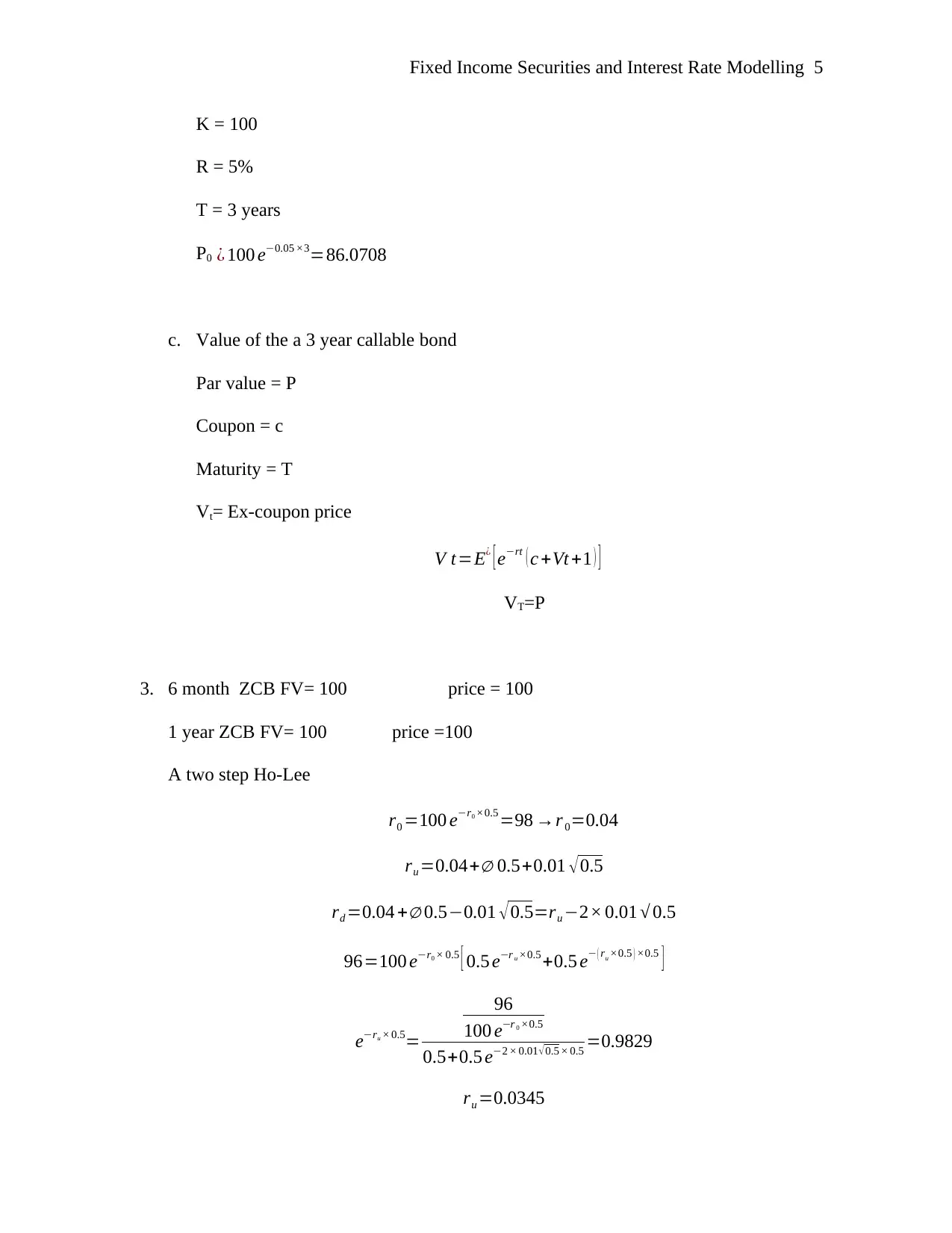
K = 100
R = 5%
T = 3 years
P0 ¿ 100 e−0.05 ×3=86.0708
c. Value of the a 3 year callable bond
Par value = P
Coupon = c
Maturity = T
Vt= Ex-coupon price
V t=E¿ [ e−rt ( c +Vt +1 ) ]
VT=P
3. 6 month ZCB FV= 100 price = 100
1 year ZCB FV= 100 price =100
A two step Ho-Lee
r0 =100 e−r0 ×0.5 =98 →r 0=0.04
ru =0.04+∅ 0.5+0.01 √ 0.5
rd =0.04 +∅ 0.5−0.01 √ 0.5=ru −2× 0.01 √ 0.5
96=100 e−r0 × 0.5 [ 0.5 e−r u ×0.5+0.5 e− ( ru ×0.5 ) ×0.5 ]
e−ru × 0.5=
96
100 e−r 0 ×0.5
0.5+0.5 e−2 × 0.01 √0.5 × 0.5 =0.9829
ru =0.0345

Fixed Income Securities and Interest Rate Modelling 6
erd
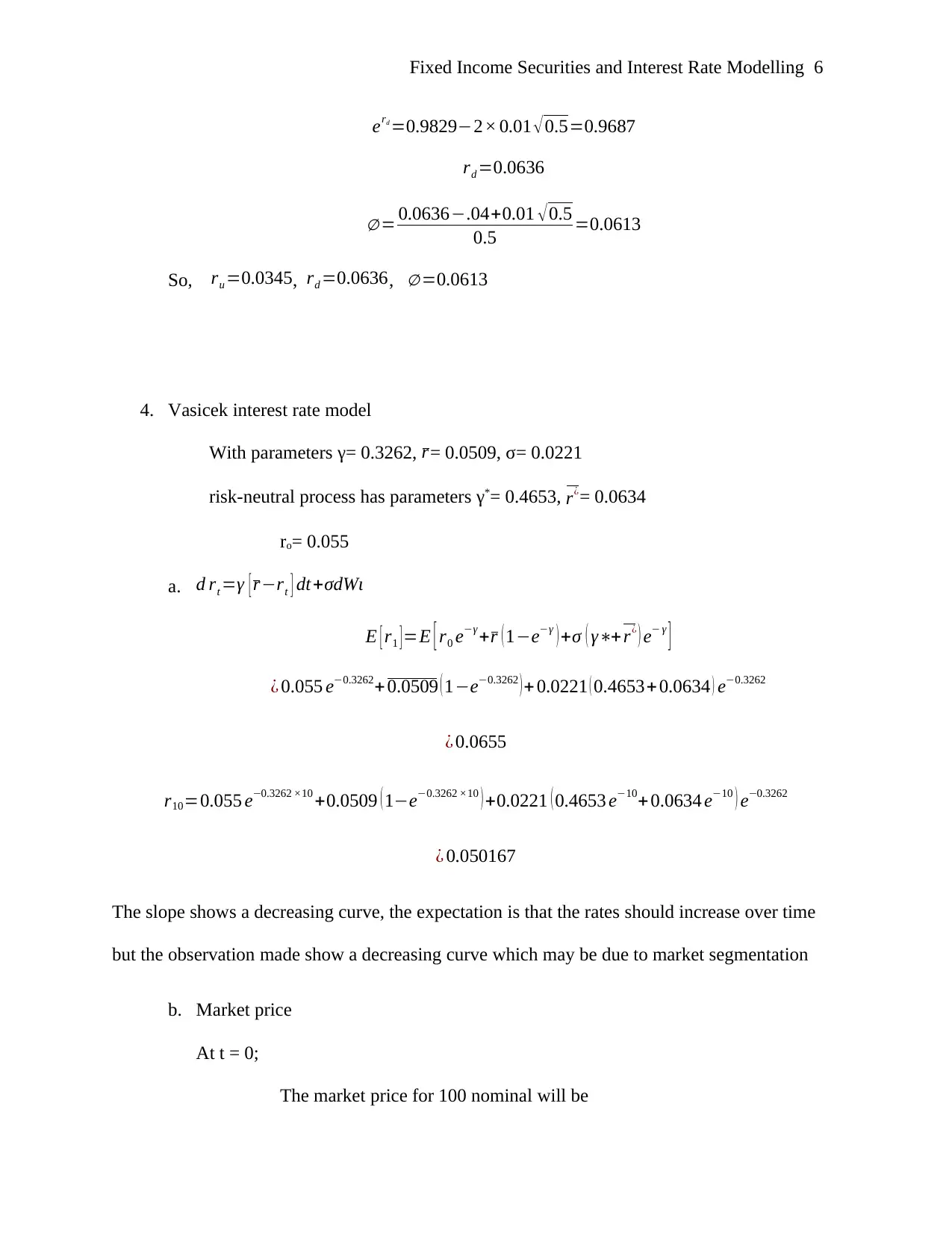
=0.9829−2× 0.01 √ 0.5=0.9687
rd =0.0636
∅ = 0.0636−.04+0.01 √0.5
0.5 =0.0613
So, ru =0.0345, rd =0.0636, ∅ =0.0613
4. Vasicek interest rate model
With parameters γ= 0.3262, r= 0.0509, σ= 0.0221
risk-neutral process has parameters γ*= 0.4653, r¿= 0.0634
ro= 0.055
a. d rt =γ [ r−rt ] dt+σdWι
Ε [ r1 ]=Ε [ r0 e−γ +r (1−e−γ ) +σ ( γ∗+r¿ ) e− γ
]
¿ 0.055 e−0.3262+ 0.0509 ( 1−e−0.3262 )+ 0.0221 ( 0.4653+ 0.0634 ) e−0.3262
¿ 0.0655
r10=0.055 e−0.3262 ×10 +0.0509 ( 1−e−0.3262 ×10 ) +0.0221 ( 0.4653 e−10+ 0.0634 e−10 ) e−0.3262
¿ 0.050167
The slope shows a decreasing curve, the expectation is that the rates should increase over time
but the observation made show a decreasing curve which may be due to market segmentation
b. Market price
At t = 0;
The market price for 100 nominal will be

Fixed Income Securities and Interest Rate Modelling 7
100 ( e−0.0655 )
¿ 93.6599
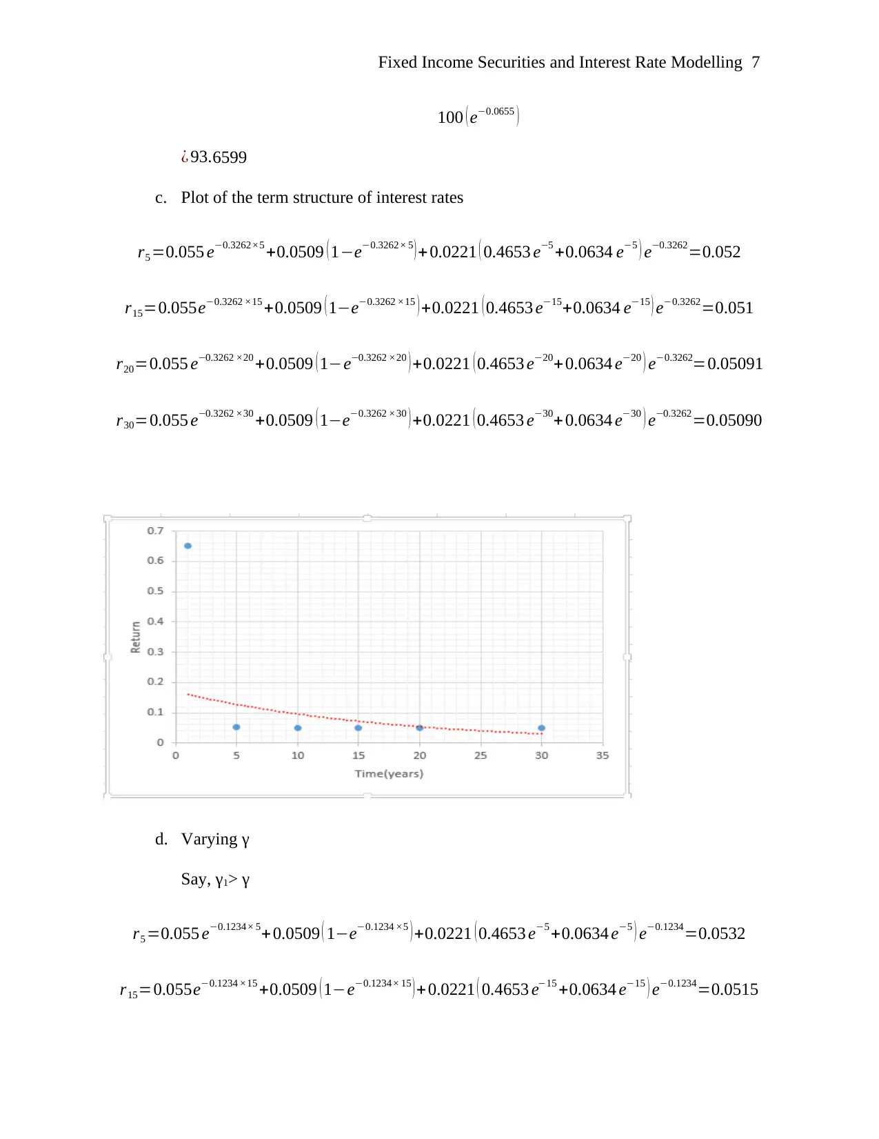
c. Plot of the term structure of interest rates
r5 =0.055 e−0.3262×5 +0.0509 ( 1−e−0.3262× 5 ) + 0.0221 ( 0.4653 e−5 +0.0634 e−5 ) e−0.3262=0.052
r15=0.055e−0.3262 ×15 +0.0509 ( 1−e−0.3262 ×15 ) +0.0221 ( 0.4653 e−15+0.0634 e−15 ) e−0.3262=0.051
r20=0.055 e−0.3262 ×20 +0.0509 ( 1−e−0.3262 ×20 ) +0.0221 ( 0.4653 e−20+0.0634 e−20 ) e−0.3262=0.05091
r30=0.055 e−0.3262 ×30 +0.0509 ( 1−e−0.3262 ×30 ) +0.0221 ( 0.4653 e−30+ 0.0634 e−30 ) e−0.3262=0.05090
d. Varying γ
Say, γ1> γ
r5 =0.055 e−0.1234× 5+ 0.0509 ( 1−e−0.1234 ×5 ) +0.0221 ( 0.4653 e−5 +0.0634 e−5 ) e−0.1234=0.0532
r15=0.055e−0.1234 ×15 +0.0509 ( 1−e−0.1234× 15 ) + 0.0221 ( 0.4653 e−15 +0.0634 e−15 ) e−0.1234=0.0515

Fixed Income Securities and Interest Rate Modelling 8
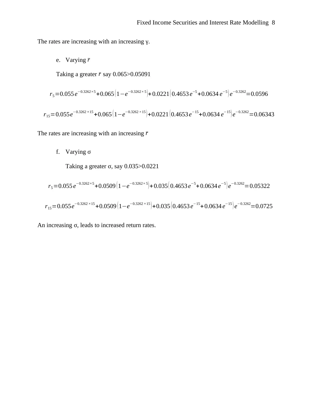
The rates are increasing with an increasing γ.
e. Varying r
Taking a greater r say 0.065>0.05091
r5 =0.055 e−0.3262×5 +0.065 ( 1−e−0.3262× 5 )+ 0.0221 ( 0.4653 e−5 +0.0634 e−5 ) e−0.3262=0.0596
r15=0.055e−0.3262 ×15 +0.065 ( 1−e−0.3262 ×15 ) +0.0221 ( 0.4653 e−15+0.0634 e−15 ) e−0.3262=0.06343
The rates are increasing with an increasing r
f. Varying σ
Taking a greater σ, say 0.035>0.0221
r5 =0.055 e−0.3262×5 +0.0509 ( 1−e−0.3262× 5 ) + 0.035 ( 0.4653 e−5+ 0.0634 e−5 ) e−0.3262=0.05322
r15=0.055e−0.3262 ×15 +0.0509 ( 1−e−0.3262 ×15 ) +0.035 ( 0.4653 e−15+0.0634 e−15 ) e−0.3262=0.0725
An increasing σ, leads to increased return rates.