Forecasting Future GDP of British Columbia using ARIMA Model

Forecasting the future GDP of British Columbia
using ARIMA model on Eviews
Student Name ******
Abstract
Basically, forecasting are important and it continually made in business, fund,
financial matters, government, and numerous different fields, and much relies on them.
Similarly, there are there are good and bad ways to forecast. The forecasting is used to
provide the great ways for current, quantitative, economic and statistical strategies for
evaluating and producing the forecasts. Forecasts are settled on to direct decisions in an
variety of fields. Gross Domestic Product (GDP) of a nation is the cash estimation of all
goods and administrations created by every one of the enterprises inside the bounds of a
nation in a year. It speaks to the total measurement of all financial action. The execution of
economy can be forecast with the assistance of GDP. As indicated by Euro stat, there are
three manners by which the GDP of a nation can be forecasts. This paper aims to displaying
and determining forecasting GDP of British Columbia utilizing ARIMA model. Here
analyzed by time series method. Auto Correlation Function (ACF) and Partial Auto
Correlation Function (PACF) are will calculated. Proper Box-Jenkins Auto Regressive
Integrated Moving Average (ARIMA) demonstrates the forecasting the future GDP of British
Columbia. Legitimacy of the model was tested using standard statistical techniques. And,
ARIMA model is used to show were utilized to forecasting zone and creation of British
Columbia for future years.
Keywords: Forecast, GDP, ACF, PACF and ARIMA
1

Introduction
The forecasting is used to provide the great ways for current, quantitative, economic
and statistical strategies for evaluating and producing the forecasts. Forecasts are settled on to
direct decisions in a variety of fields. Gross Domestic Product (GDP) of a nation is the cash
estimation of all goods and administrations created by every one of the enterprises inside the
bounds of a nation in a year. The execution of economy can be forecast with the assistance of
GDP. This paper aims to displaying and determining forecasting GDP of British Columbia
utilizing ARIMA model. Here analyzed by time series method. Auto Correlation Function
(ACF) and Partial Auto Correlation Function (PACF) are will calculated. Proper Box-Jenkins
Auto Regressive Integrated Moving Average (ARIMA) demonstrates the forecasting the
future GDP of British Columbia. Legitimacy of the model was tested using standard
statistical techniques. And, ARIMA model is used to show were utilized to forecasting zone
and creation of British Columbia for future years.
Research Objectives
1. To test the stationary in the data of GDP using the Augmented Dickey – Fullers unit
root test over the period.
2. To study Auto correlation in the observed series of GDP ACF and PACF values and
correlogram will be used to measure the AR and MA to predict which past series is a
fitter model for future value prediction.
3. To test the model validity statically a portmanteau test of Independence i.e. the BDS
test for time-based dependence in a series will be applied.
4. Finally Forecast the GDP for the next ten years using ARIMA Model along with the
upper control level (UCL) and the lower control level (LCL).
Literature Review
According to this paper (Dritsaki, 2015), the ARIMA model has be used extensively
by many researchers. This method is used to highlight the future rates of GDP. It easily
examines the forecasting of GDP growth rate for India using the ARIMA model. This model
is used to predicted the values follow an increasing the trend for a years. It establishes the
stationary of time series. Result of this paper is used to provide the policy makers to
formulate the effective policies for attracting the foreign direct investment. It also helpful the
2

managerial business executive for implementing or taking decision concerned with the
expansion of the existing business.
Methodology
The GDP data was collected over the time period from 1997 to 2017 were used for
forecasting the future values using Auto Regressive Integrated Moving Average (ARIMA)
models. The ARIMA procedure is likewise called as Box-Jenkins approach. The Box-Jenkins
method is worried about fitting an ARIMA model to a given data of information. The
objective in fitting ARIMA model is to distinguish the stochastic procedure of the time series
and predicted the future values correctly. These strategies have additionally been helpful in
numerous sorts of circumstances which include the working of models for discrete time series
and dynamic frameworks. Anyway this technique is not useful for seasonal series with a large
random component.
Data Description
The GDP data was collected over the time period from 1997 to 2017. The provided data was
contains the information about the forecast the GDP growth for the province of British
Columbia based on the overall annual expenditure. It is illustrated as below (Camacho &
Martinez-Martin, 2013).
3

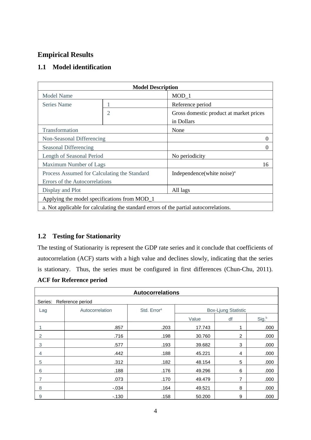
Empirical Results
1.1 Model identification
Model Description
Model Name MOD_1
Series Name 1 Reference period
2 Gross domestic product at market prices
in Dollars
Transformation None
Non-Seasonal Differencing 0
Seasonal Differencing 0
Length of Seasonal Period No periodicity
Maximum Number of Lags 16
Process Assumed for Calculating the Standard
Errors of the Autocorrelations
Independence(white noise)a
Display and Plot All lags
Applying the model specifications from MOD_1
a. Not applicable for calculating the standard errors of the partial autocorrelations.
1.2 Testing for Stationarity
The testing of Stationarity is represent the GDP rate series and it conclude that coefficients of
autocorrelation (ACF) starts with a high value and declines slowly, indicating that the series
is stationary. Thus, the series must be configured in first differences (Chun-Chu, 2011).
ACF for Reference period
Autocorrelations
Series: Reference period
Lag Autocorrelation Std. Errora Box-Ljung Statistic
Value df Sig.b
1 .857 .203 17.743 1 .000
2 .716 .198 30.760 2 .000
3 .577 .193 39.682 3 .000
4 .442 .188 45.221 4 .000
5 .312 .182 48.154 5 .000
6 .188 .176 49.296 6 .000
7 .073 .170 49.479 7 .000
8 -.034 .164 49.521 8 .000
9 -.130 .158 50.200 9 .000
4

References

Camacho, M., & Martinez-Martin, J. (2013). Real-time forecasting US GDP from small-scale
factor models. Empirical Economics, 47(1), 347-364. doi: 10.1007/s00181-013-0731-4
Chun-Chu. (2011). Forecasting the Spanish Stock Market Returns with Fractional and Non-
Fractional Models. American Journal Of Economics And Business Administration, 3(4),
586-588. doi: 10.3844/ajebasp.2011.586.588
Dritsaki, D. (2015). Forecasting Real GDP Rate through Econometric Models: An Empirical
Study from Greece. Journal Of International Business And Economics, 3(1). doi:
10.15640/jibe.v3n1a2
Fildes, R., & Allen, P. (2011). Forecasting. Los Angeles, Calif.: SAGE.
11
Şen Doğan, B., & Midiliç, M. (2018). Forecasting Turkish real GDP growth in a data-rich
environment. Empirical Economics. doi: 10.1007/s00181-017-1357-8
12
⊘ This is a preview!⊘
Do you want full access?
Subscribe today to unlock all pages.
Trusted by 1+ million students worldwide
1 out of 12
Your All-in-One AI-Powered Toolkit for Academic Success.
+13062052269
info@desklib.com
Available 24*7 on WhatsApp / Email
![[object Object]](/_next/static/media/star-bottom.7253800d.svg)
Unlock your academic potential
Copyright © 2020–2025 A2Z Services. All Rights Reserved. Developed and managed by ZUCOL.