Time Series Forecasting and Regression Analysis Assignment
VerifiedAdded on 2022/10/11
|12
|1735
|7
Practical Assignment
AI Summary
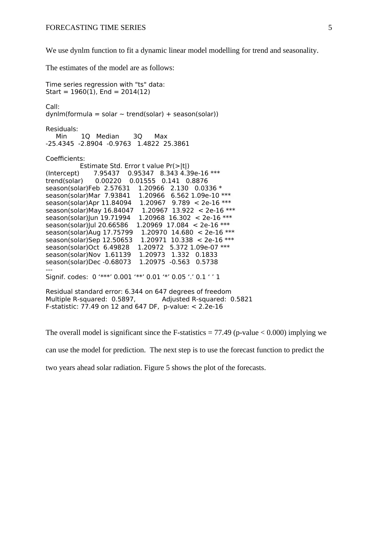
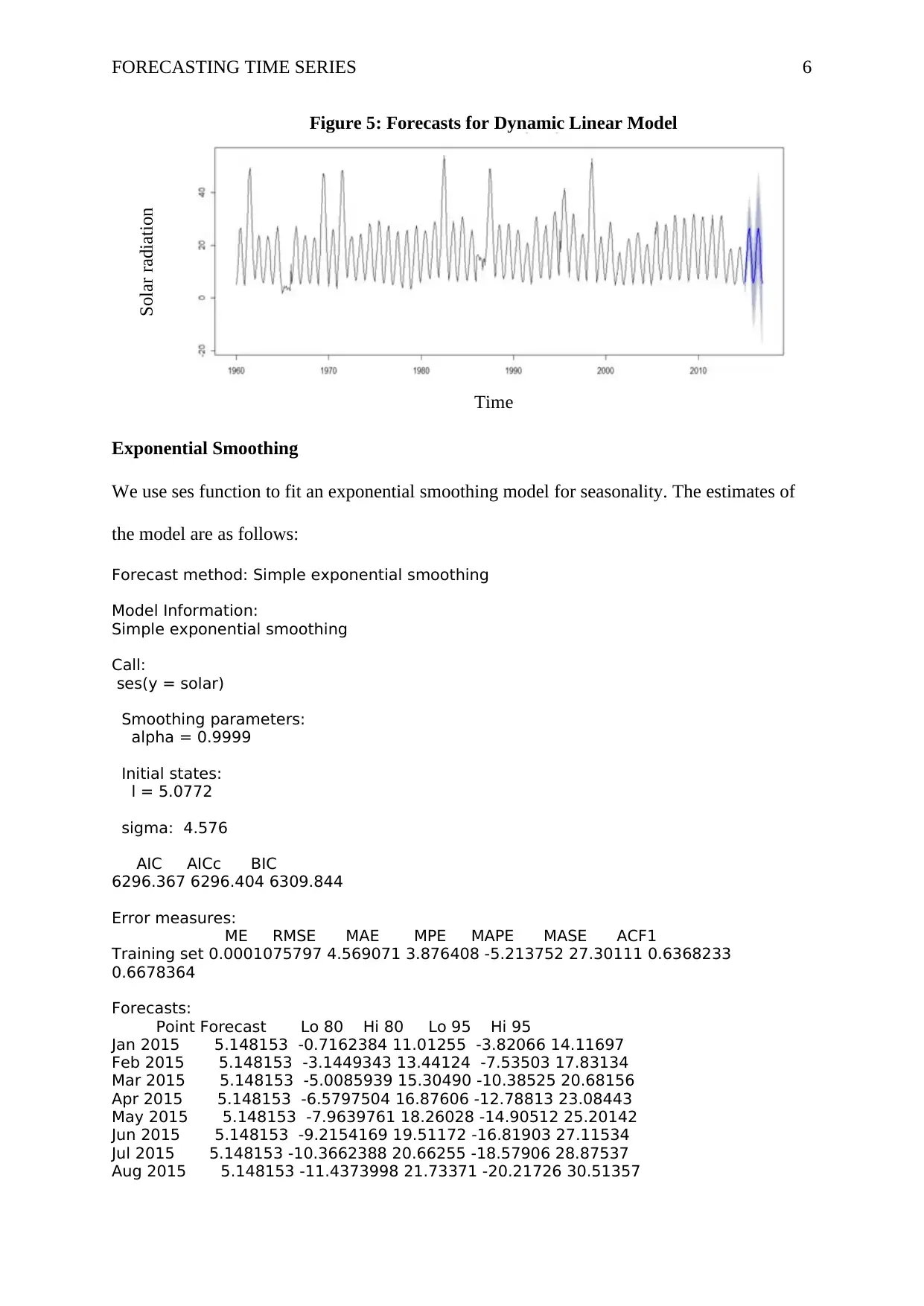
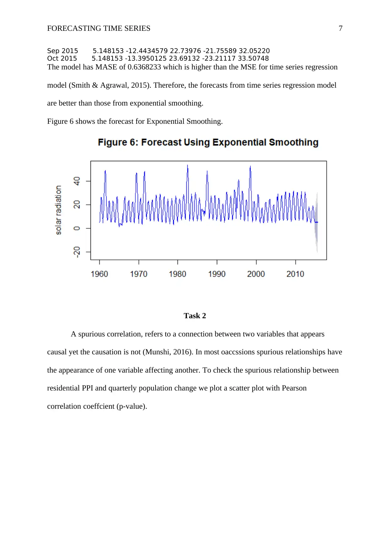
This assignment focuses on time series forecasting using R programming. Task 1 involves analyzing and forecasting monthly average horizontal solar radiation data using time series regression methods (dLagM package), dynamic linear models (dynlm package), and exponential smoothing. The analysis includes data exploration, stationarity testing, model fitting, and forecasting for two years ahead, with model comparison based on MASE. Task 2 explores spurious correlation between residential PPI and quarterly population change, involving scatter plot analysis and correlation coefficient calculation. The assignment utilizes various R packages for data manipulation, model building, and visualization, providing a comprehensive approach to time series analysis and forecasting techniques. The solution includes R codes, plots, and interpretations of the results, demonstrating the application of different forecasting methods and the identification of spurious relationships in time series data.

1 out of 12
Related Documents


Your All-in-One AI-Powered Toolkit for Academic Success.
+13062052269
info@desklib.com
Available 24*7 on WhatsApp / Email
![[object Object]](/_next/static/media/star-bottom.7253800d.svg)
Copyright © 2020–2026 A2Z Services. All Rights Reserved. Developed and managed by ZUCOL.