Comprehensive Statistical Analysis for Business Applications
VerifiedAdded on 2023/04/22
|12
|1656
|428
Homework Assignment
AI Summary
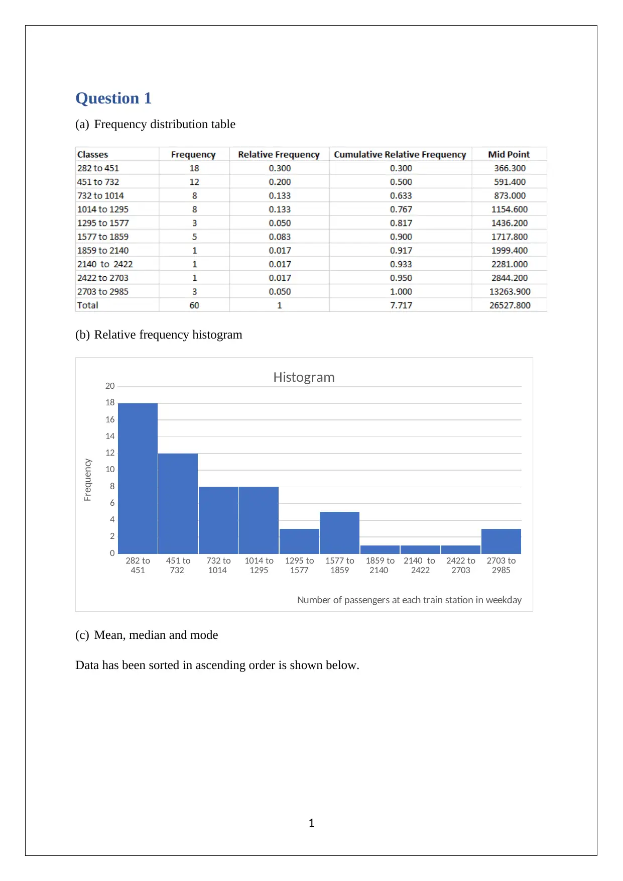
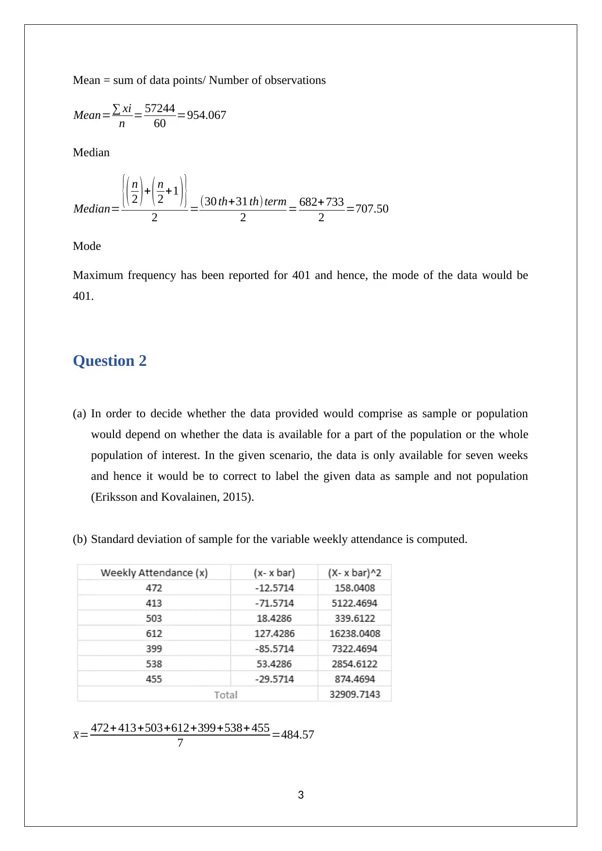
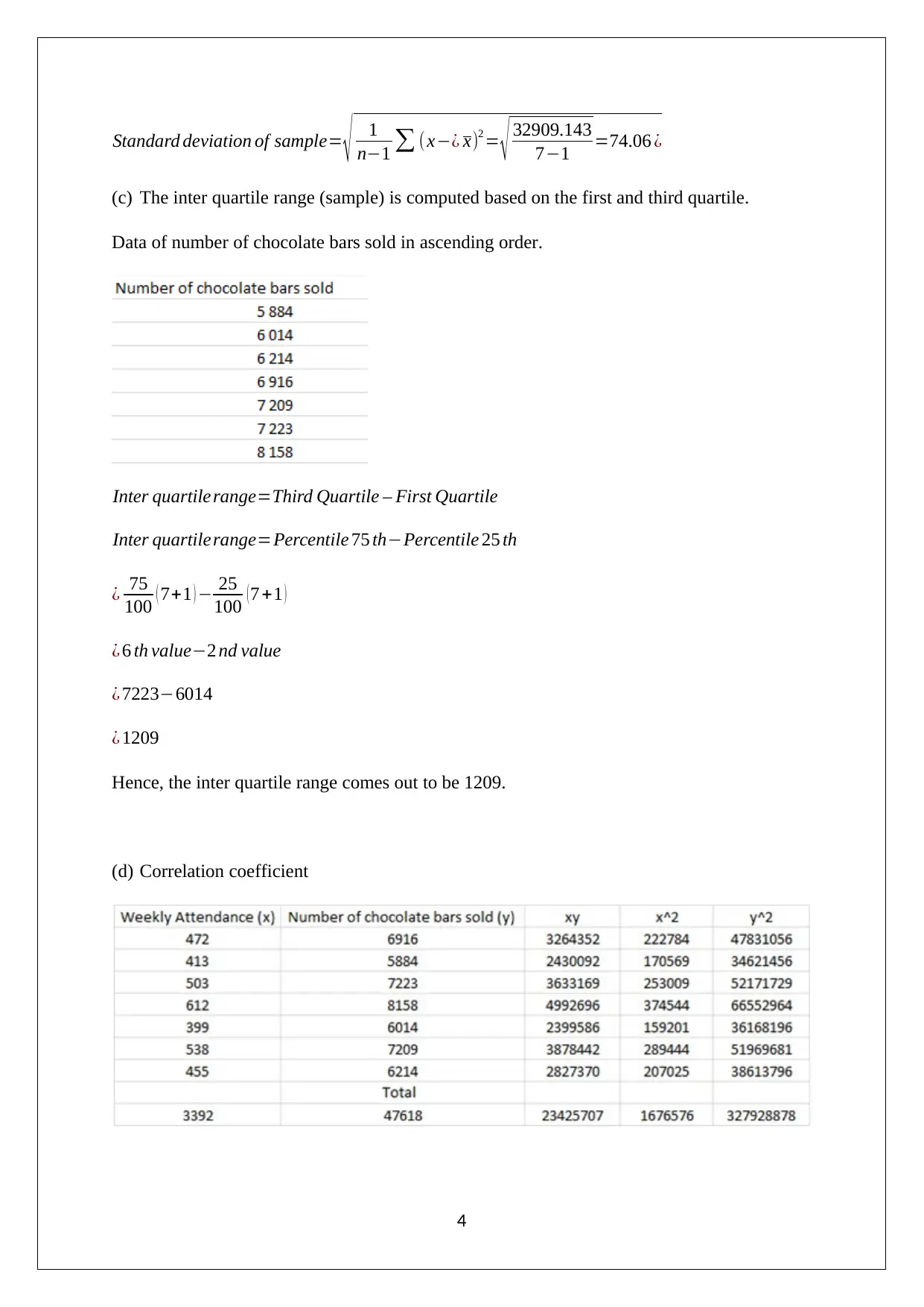
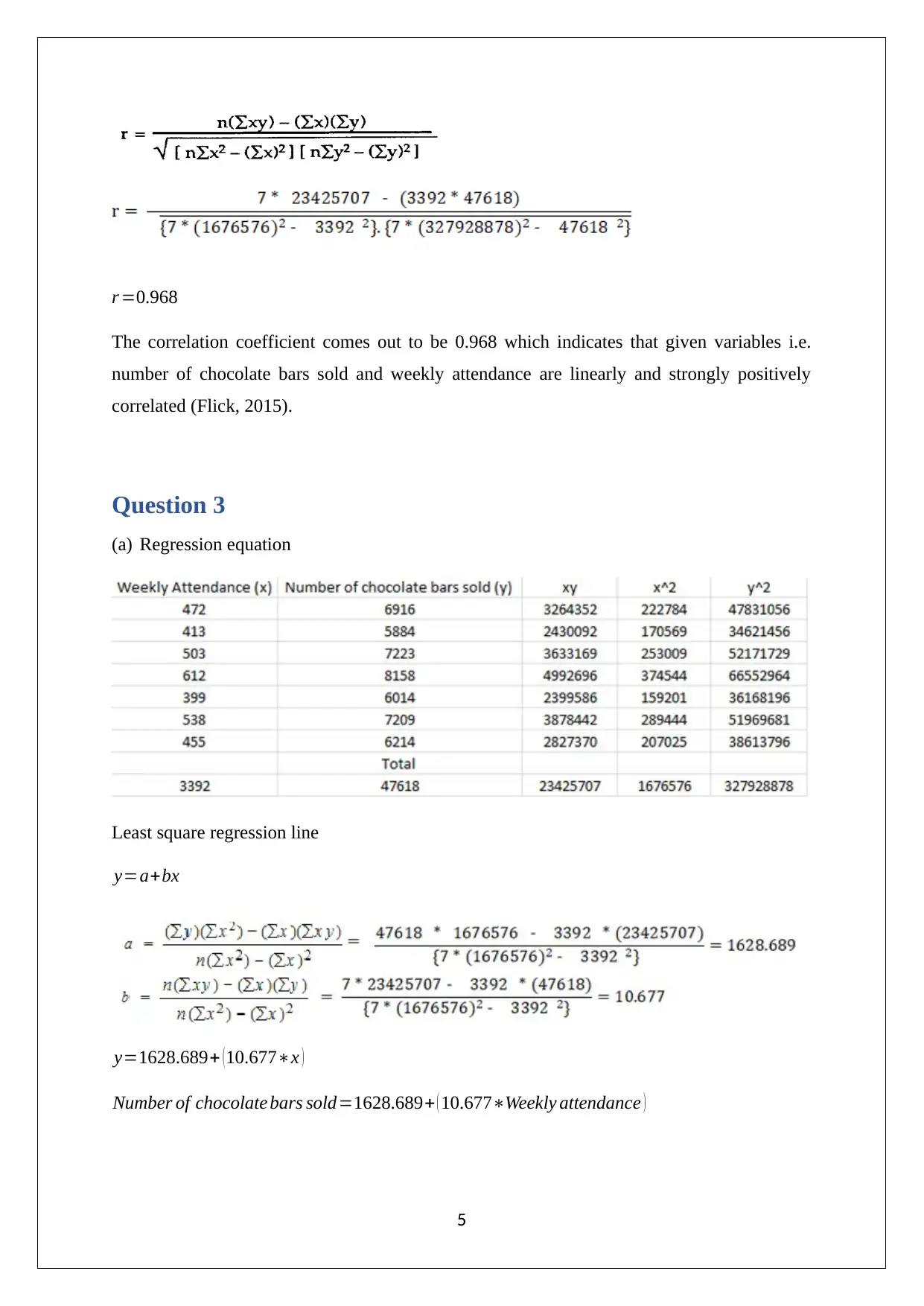
This assignment provides comprehensive solutions to various statistical problems relevant to business applications. It includes the creation of a frequency distribution table and relative frequency histogram, calculation of mean, median, and mode, and determination of sample standard deviation and interquartile range. The assignment also covers correlation coefficient analysis, regression equation derivation, and coefficient of determination interpretation. Furthermore, it addresses probability calculations, including conditional probabilities and independence testing. The document also includes binomial and Poisson distribution problems and normal distribution calculations related to average selling prices. The final question discusses the selection of appropriate statistical tests based on sample size and calculates probabilities related to investor proportions. This assignment showcases a strong understanding of statistical methods and their application in business contexts. Desklib offers a variety of similar solved assignments and past papers to aid students in their studies.

STATISTICS
[DATE]
[DATE]
Paraphrase This Document
Need a fresh take? Get an instant paraphrase of this document with our AI Paraphraser

Question 1
(a) Frequency distribution table
(b) Relative frequency histogram
282 to
451 451 to
732 732 to
1014 1014 to
1295 1295 to
1577 1577 to
1859 1859 to
2140 2140 to
2422 2422 to
2703 2703 to
2985
0
2
4
6
8
10
12
14
16
18
20 Histogram
Number of passengers at each train station in weekday
Frequency
(c) Mean, median and mode
Data has been sorted in ascending order is shown below.
1

2
⊘ This is a preview!⊘
Do you want full access?
Subscribe today to unlock all pages.

Trusted by 1+ million students worldwide

Mean = sum of data points/ Number of observations
Mean=∑ xi
n = 57244
60 =954.067
Median
Median= {( n
2 )+ ( n
2 +1 ) }
2 =(30 th+31 th) term
2 = 682+ 733
2 =707.50
Mode
Maximum frequency has been reported for 401 and hence, the mode of the data would be
401.
Question 2
(a) In order to decide whether the data provided would comprise as sample or population
would depend on whether the data is available for a part of the population or the whole
population of interest. In the given scenario, the data is only available for seven weeks
and hence it would be to correct to label the given data as sample and not population
(Eriksson and Kovalainen, 2015).
(b) Standard deviation of sample for the variable weekly attendance is computed.
x= 472+ 413+503+612+399+538+ 455
7 =484.57
3
Paraphrase This Document
Need a fresh take? Get an instant paraphrase of this document with our AI Paraphraser

Standard deviation of sample= √ 1
n−1 ∑ (x−¿ x)2 = √ 32909.143
7−1 =74.06 ¿
(c) The inter quartile range (sample) is computed based on the first and third quartile.
Data of number of chocolate bars sold in ascending order.
Inter quartile range=Third Quartile – First Quartile
Inter quartilerange=Percentile 75 th−Percentile 25 th
¿ 75
100 ( 7+1 ) − 25
100 (7 +1 )
¿ 6 th value−2 nd value
¿ 7223−6014
¿ 1209
Hence, the inter quartile range comes out to be 1209.
(d) Correlation coefficient
4

r =0.968
The correlation coefficient comes out to be 0.968 which indicates that given variables i.e.
number of chocolate bars sold and weekly attendance are linearly and strongly positively
correlated (Flick, 2015).
Question 3
(a) Regression equation
Least square regression line
y=a+bx
y=1628.689+ ( 10.677∗x )
Number of chocolate bars sold=1628.689+ ( 10.677∗Weekly attendance )
5
⊘ This is a preview!⊘
Do you want full access?
Subscribe today to unlock all pages.

Trusted by 1+ million students worldwide

Example
(1) When Holmes is closed then the weekly attendance of the student would be zero.
Hence,
Number of chocolate bars sold=1628.689+ ( 10.677∗Weekly attendance )
Number of chocolate bars sold=1628.689+ ( 10.677∗0 ) =1629bars of chocolate
(2) When the independent variable is increased by 10 times (number of students has
increased by 10 times) then the total sales of number of chocolate bars has also increased
by (10*10.67) = 1067. The total number of chocolate bars sold would be calculated after
considering the effect of 10 which is (10*10.67).
(3) Coefficient of determination
The coefficient of determination is square of correlation coefficient.
Correlation coefficient=0.968
R2= ( 0.968 )2=0.937
Coefficient of determination comes out to be 0.937which indicates that 93.7% of variation in
the number of chocolate bars sold can be explained by variation in the weekly attendance of
the students. The value is close to 1 which implies that regression model is good fit (Hillier,
2016).
Question 4
The information and data are highlighted below.
(a) Probability that a randomly selected player would be from Holmes OR would receive
Grassroots training.
6
Paraphrase This Document
Need a fresh take? Get an instant paraphrase of this document with our AI Paraphraser

P= 35+92+12
35+92+54 +12
P= 139
193 =0.720
(b) Probability that a randomly selected player would be External AND would receive
scientific training.
P= 54
35+92+54 +12
P= 54
193 =0.28
(c) Probability that a player is from Holmes who is receiving scientific training.
P= 35
35+92
P= 35
127 =0.276
(d) Training and recruitment are independent or not.
Let event A is Training and event B is Recruitment.
Event A and B would be independent when P( A) . P( B)=P( A∧B)
Now,
P ( A∧B )=0.2570
P ( A )= 54+12
( 35+92+54 +12 ) =0.341
P ( B ) = 35+54
( 35+92+54+12 ) =0.461
P ( A )∗P ( B )=0.341∗0.461=0.157
It can be seen from the above that P( A). P(B) ≠ P( A∧B) and hence, the required condition
for events being independent is not satisfied and hence, Training and Recruitments are not
independent events.
7
35+92+54 +12
P= 139
193 =0.720
(b) Probability that a randomly selected player would be External AND would receive
scientific training.
P= 54
35+92+54 +12
P= 54
193 =0.28
(c) Probability that a player is from Holmes who is receiving scientific training.
P= 35
35+92
P= 35
127 =0.276
(d) Training and recruitment are independent or not.
Let event A is Training and event B is Recruitment.
Event A and B would be independent when P( A) . P( B)=P( A∧B)
Now,
P ( A∧B )=0.2570
P ( A )= 54+12
( 35+92+54 +12 ) =0.341
P ( B ) = 35+54
( 35+92+54+12 ) =0.461
P ( A )∗P ( B )=0.341∗0.461=0.157
It can be seen from the above that P( A). P(B) ≠ P( A∧B) and hence, the required condition
for events being independent is not satisfied and hence, Training and Recruitments are not
independent events.
7

Question 5
(a) Requisite probability that the customer will select product x from A segment
P ( A |X ) = P ( A )∗P ( X |A )
P ( X ) = ( 0.55 )∗ ( 0.2 )
( 0.55∗0.2 )+ ( 0.35∗0.3 )+ ( 0.6∗0.1 )+ ( 0.9∗0.05 ) =0.3537
Requisite probability that the customer will select product x
P ( X ) =¿
Question 6
Let, x is total number of customers enter in the shop and p is the number of customers who
will surely purchase from the shop.
(a) Probability that 2 or lesser than 2 customers will surely purchase from the shop
Distribution: Binomial Distribution
P ( X=x ) = n !
x ! ( n−x ) ! pX (1− p)n− X
In present case, n=8 , p=0.1 x=0,1 , 2
Now,
P ( x ≤ 2 ) =P ( x=2 ) + P ( x =1 ) + P ( x=0)
P( x ≤2)= { 8!
2 ! ( 8−2 ) ! ( 0.1 ) 8 ( 1−0.1 ) 8−2
}+ { 8 !
1 ! ( 8−1 ) ! ( 0.1 ) 8 ( 1−0.1 ) 8−1
}+ { 8 !
0 ! ( 8−0 ) ! ( 0.1 ) 8 ( 1−0.1 )8 −0
}
8
⊘ This is a preview!⊘
Do you want full access?
Subscribe today to unlock all pages.

Trusted by 1+ million students worldwide

P ( x ≤ 2 )=0.1488+0.3826 +0.4304=0.9619
There is a 0.9619 probability that 2 or lesser than 2 customers will surely purchase from the
shop.
(b) Probability that 9 customers enters in shop within 2 minutes
Distribution: Poisson Distribution
P( X=x)= e−γ γx
x !
In present case, x=9 , γ=8
P ( X=9 ) = e−8 89
(9)! =0.124
There is a 0.124 probability that 9 customers enter in shop within 2 minutes.
Question 7
Average selling price = $1.1 million
Standard deviation = $385,000
Distribution: Normally distributed
(a) Probability that apartment would be sold for over $2 million
P ( x>2000000 ) =P ( 2000000−1100000
385000 ) =P ( Z >2.340 )
Based on Normal Distribution Table
P ( x>2000000 )=P ( Z >2.340 ) =0.00970
(b) Probability that apartment would be sold for over $1 million but would be lesser than $1.1
million
9
Paraphrase This Document
Need a fresh take? Get an instant paraphrase of this document with our AI Paraphraser

P ( 1000000< x<1100000 )=P ( 1000000−1100000
385000 <x< 11000000−1000000
385000 )
P ( 1000000< x<1100000 ) P ( −0.26< z <0.0 ) =0.3975−0.50=0.1025
Question 8
(a) The selection of t statistic or z statistic depends on the sample size. According to Central
Limit Theorem, the minimum sample size needed for normal distribution is 30. Hence,
when the sample size is higher than 30 then the distribution would assume to be normal
and z statistic would be taken into consideration. In present case, the sample of 50
properties is present and therefore, z statistic would be used and distribution would be
assumed to be normally distributed (Hair et. al., 2015).
(b) Total number of investors = 45
Number of investors which are agree to do investment = 11
Total proportion of agreed investors p= 11
45 =0.240
Standard error S . E .= √ p ( 1− p )
n = √ 0.240 ( 1−0.240 )
45 =0.0640
Probability that proportion would be higher than 30% is computed as shown below.
P ( p >30 % ) =P (Z> x−μ
S . E . )
P ( p >30 % ) =P (Z> 0.30−0.240
0.0640 )
P ( p >30 % ) =P ( Z >0.870 )
Based on Normal Distribution Table
P ( p >30 % ) =P ( Z >0.870 )=0.1920
Hence, the requisite probability would be 0.1920.
References
10

Eriksson, P. and Kovalainen, A. (2015). Quantitative methods in business research (3rd ed.).
London: Sage Publications, pp. 65-66
Flick, U. (2015). Introducing research methodology: A beginner's guide to doing a research
project (4th ed.). New York: Sage Publications, pp.76
Hair, J. F., Wolfinbarger, M., Money, A. H., Samouel, P., and Page, M. J. (2015). Essentials
of business research methods (2nd ed.). New York: Routledge, pp.84-85
Hillier, F. (2016). Introduction to Operations Research. (6th ed.). New York: McGraw Hill
Publications, pp. 59
11
⊘ This is a preview!⊘
Do you want full access?
Subscribe today to unlock all pages.

Trusted by 1+ million students worldwide
1 out of 12