Statistical Analysis of Fruit Production Data - Biostatistics

This report presents statistical analysis of fruit production data including descriptive and inferential analysis. The aim of this report was to present statistical analysis of fruit production data. The data consisted of four variables three of which were categorical variables while one variable was a quantitative variable.

Biostatistics
Name:
Institution:
29th May 2018

Introduction
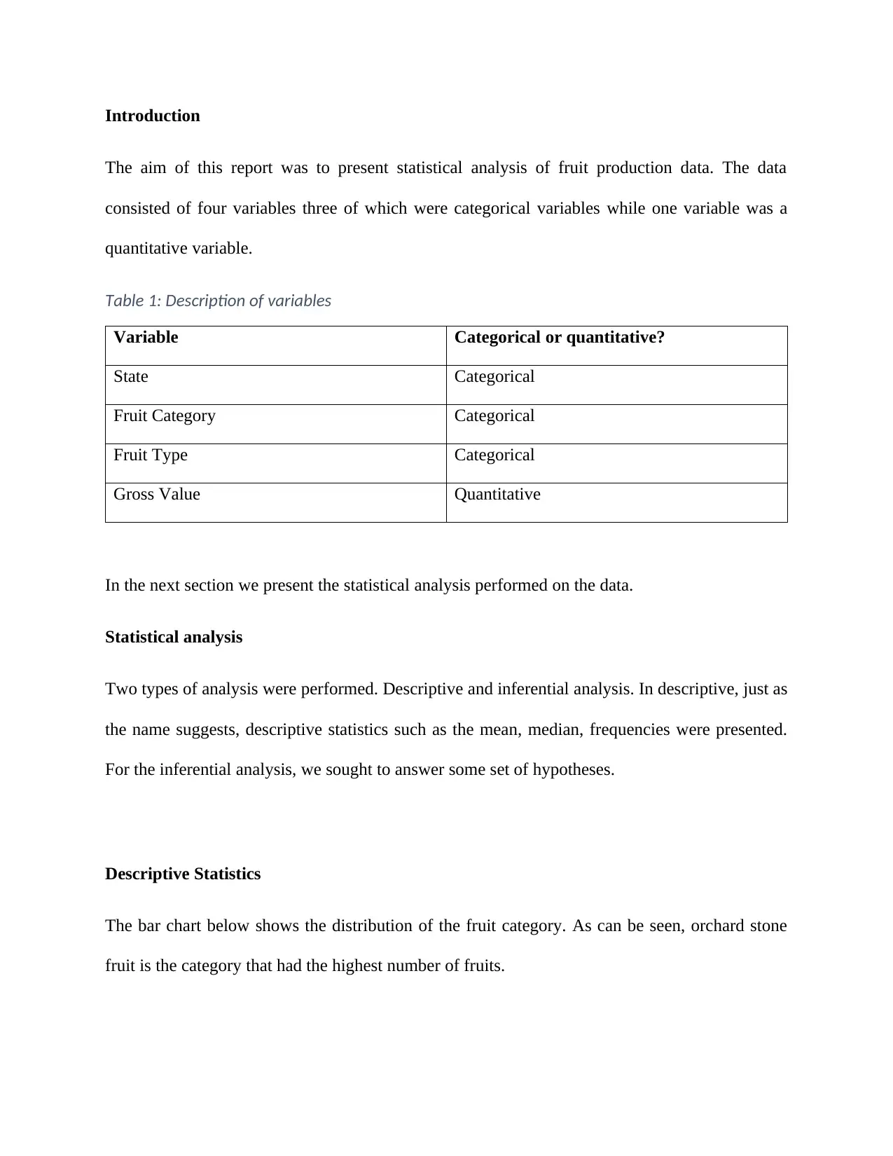
The aim of this report was to present statistical analysis of fruit production data. The data
consisted of four variables three of which were categorical variables while one variable was a
quantitative variable.
Table 1: Description of variables
Variable Categorical or quantitative?
State Categorical
Fruit Category Categorical
Fruit Type Categorical
Gross Value Quantitative
In the next section we present the statistical analysis performed on the data.
Statistical analysis
Two types of analysis were performed. Descriptive and inferential analysis. In descriptive, just as
the name suggests, descriptive statistics such as the mean, median, frequencies were presented.
For the inferential analysis, we sought to answer some set of hypotheses.
Descriptive Statistics
The bar chart below shows the distribution of the fruit category. As can be seen, orchard stone
fruit is the category that had the highest number of fruits.

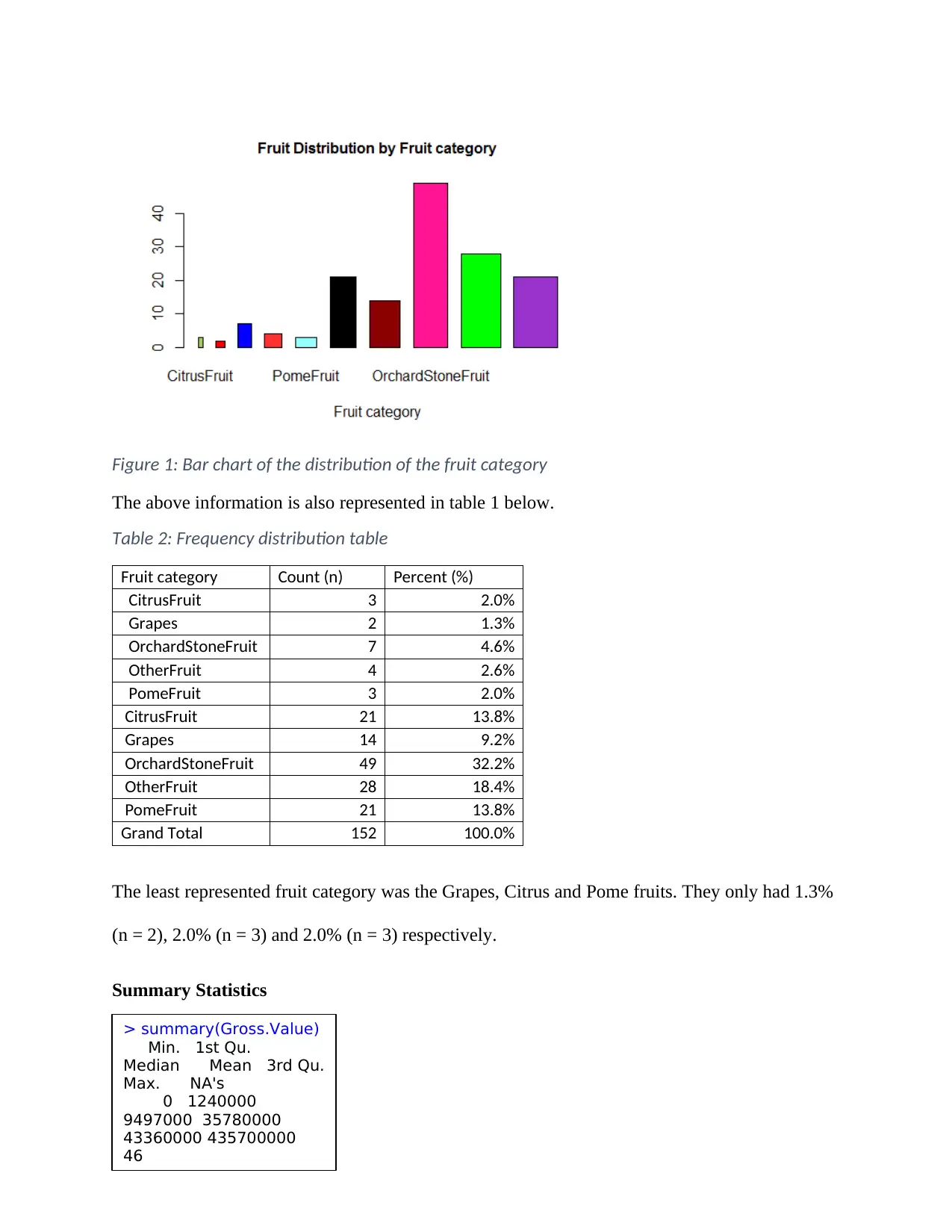
Figure 1: Bar chart of the distribution of the fruit category
The above information is also represented in table 1 below.
Table 2: Frequency distribution table
Fruit category Count (n) Percent (%)
CitrusFruit 3 2.0%
Grapes 2 1.3%
OrchardStoneFruit 7 4.6%
OtherFruit 4 2.6%
PomeFruit 3 2.0%
CitrusFruit 21 13.8%
Grapes 14 9.2%
OrchardStoneFruit 49 32.2%
OtherFruit 28 18.4%
PomeFruit 21 13.8%
Grand Total 152 100.0%
The least represented fruit category was the Grapes, Citrus and Pome fruits. They only had 1.3%
(n = 2), 2.0% (n = 3) and 2.0% (n = 3) respectively.
Summary Statistics
> summary(Gross.Value)
Min. 1st Qu.
Median Mean 3rd Qu.
Max. NA's
0 1240000
9497000 35780000
43360000 435700000
46

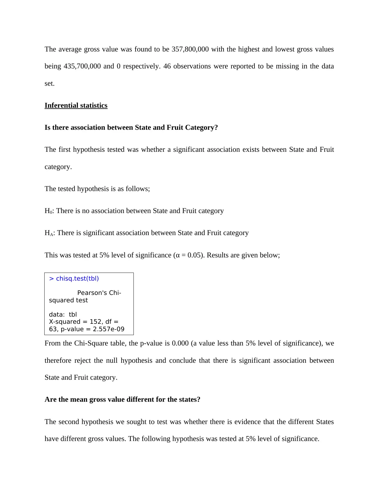
The average gross value was found to be 357,800,000 with the highest and lowest gross values
being 435,700,000 and 0 respectively. 46 observations were reported to be missing in the data
set.
Inferential statistics
Is there association between State and Fruit Category?
The first hypothesis tested was whether a significant association exists between State and Fruit
category.
The tested hypothesis is as follows;
H0: There is no association between State and Fruit category
HA: There is significant association between State and Fruit category
This was tested at 5% level of significance (α = 0.05). Results are given below;
From the Chi-Square table, the p-value is 0.000 (a value less than 5% level of significance), we
therefore reject the null hypothesis and conclude that there is significant association between
State and Fruit category.
Are the mean gross value different for the states?
The second hypothesis we sought to test was whether there is evidence that the different States
have different gross values. The following hypothesis was tested at 5% level of significance.
> chisq.test(tbl)
Pearson's Chi-
squared test
data: tbl
X-squared = 152, df =
63, p-value = 2.557e-09

H0: The means gross values is the same for all the States
HA: At least one of the States has a different mean gross value.
α = 0.05
To test the above hypothesis, a one way analysis of variance (ANOVA) test was performed
(Gelman, 2005). The test (ANOVA) is a statistical test that is used to test for mean differences in
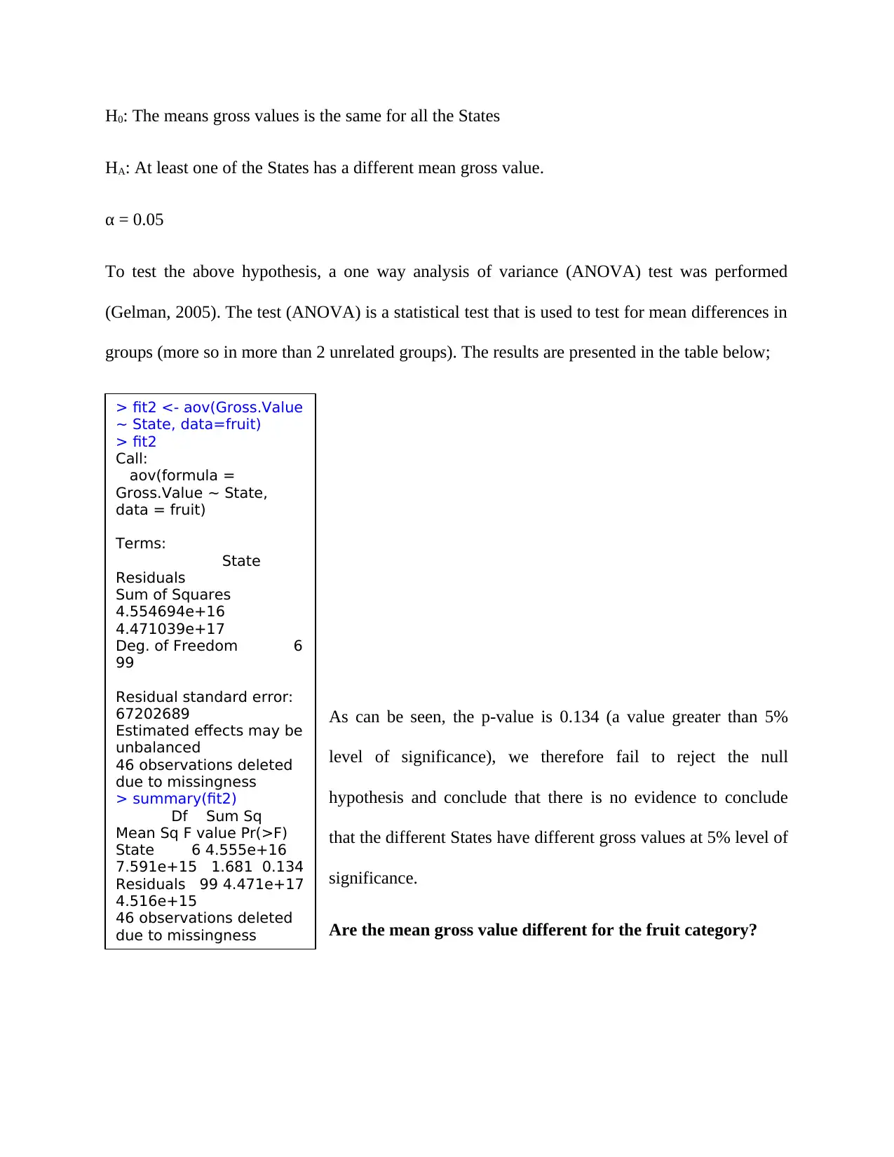
groups (more so in more than 2 unrelated groups). The results are presented in the table below;
As can be seen, the p-value is 0.134 (a value greater than 5%
level of significance), we therefore fail to reject the null
hypothesis and conclude that there is no evidence to conclude
that the different States have different gross values at 5% level of
significance.
Are the mean gross value different for the fruit category?
> fit2 <- aov(Gross.Value
~ State, data=fruit)
> fit2
Call:
aov(formula =
Gross.Value ~ State,
data = fruit)
Terms:
State
Residuals
Sum of Squares
4.554694e+16
4.471039e+17
Deg. of Freedom 6
99
Residual standard error:
67202689
Estimated effects may be
unbalanced
46 observations deleted
due to missingness
> summary(fit2)
Df Sum Sq
Mean Sq F value Pr(>F)
State 6 4.555e+16
7.591e+15 1.681 0.134
Residuals 99 4.471e+17
4.516e+15
46 observations deleted
due to missingness

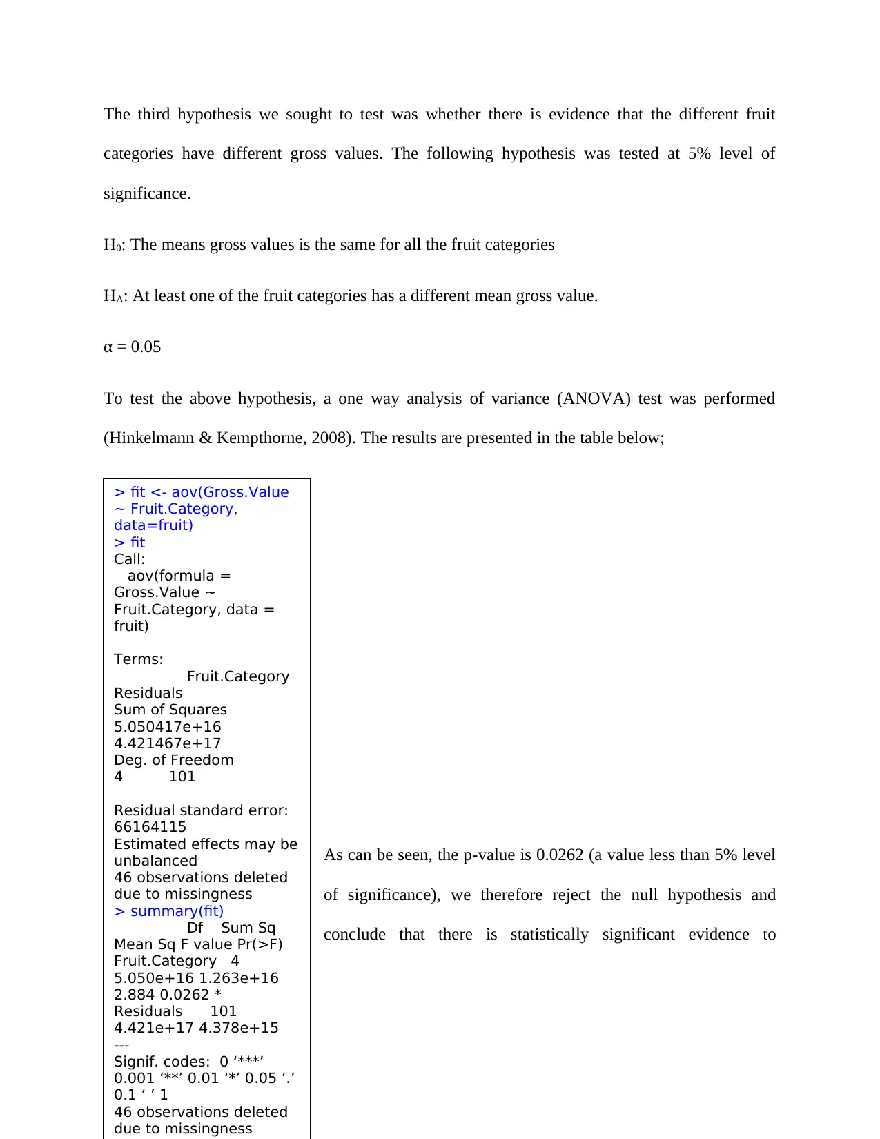
The third hypothesis we sought to test was whether there is evidence that the different fruit
categories have different gross values. The following hypothesis was tested at 5% level of
significance.
H0: The means gross values is the same for all the fruit categories
HA: At least one of the fruit categories has a different mean gross value.
α = 0.05
To test the above hypothesis, a one way analysis of variance (ANOVA) test was performed
(Hinkelmann & Kempthorne, 2008). The results are presented in the table below;
As can be seen, the p-value is 0.0262 (a value less than 5% level
of significance), we therefore reject the null hypothesis and
conclude that there is statistically significant evidence to
> fit <- aov(Gross.Value
~ Fruit.Category,
data=fruit)
> fit
Call:
aov(formula =
Gross.Value ~
Fruit.Category, data =
fruit)
Terms:
Fruit.Category
Residuals
Sum of Squares
5.050417e+16
4.421467e+17
Deg. of Freedom
4 101
Residual standard error:
66164115
Estimated effects may be
unbalanced
46 observations deleted
due to missingness
> summary(fit)
Df Sum Sq
Mean Sq F value Pr(>F)
Fruit.Category 4
5.050e+16 1.263e+16
2.884 0.0262 *
Residuals 101
4.421e+17 4.378e+15
---
Signif. codes: 0 ‘***’
0.001 ‘**’ 0.01 ‘*’ 0.05 ‘.’
0.1 ‘ ’ 1
46 observations deleted
due to missingness

conclude that at least one of the fruit categories has a significantly different mean gross value at
5% level of significance.
References
Gelman, A., 2005. Analysis of variance? Why it is more important than ever. The Annals of
Statistics, 33(5), p. 1–53.
Hinkelmann , S. & Kempthorne, B., 2008. Completely Randomized Design; Derived Linear
Model. Volume 1.

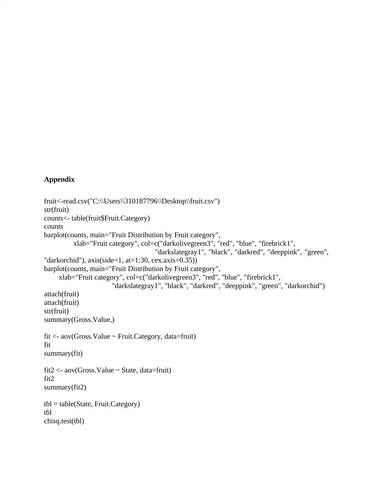
Appendix
fruit<-read.csv("C:\\Users\\310187796\\Desktop\\fruit.csv")
str(fruit)
counts<- table(fruit$Fruit.Category)
counts
barplot(counts, main="Fruit Distribution by Fruit category",
xlab="Fruit category", col=c("darkolivegreen3", "red", "blue", "firebrick1",
"darkslategray1", "black", "darkred", "deeppink", "green",
"darkorchid"), axis(side=1, at=1:30, cex.axis=0.35))
barplot(counts, main="Fruit Distribution by Fruit category",
xlab="Fruit category", col=c("darkolivegreen3", "red", "blue", "firebrick1",
"darkslategray1", "black", "darkred", "deeppink", "green", "darkorchid")
attach(fruit)
attach(fruit)
str(fruit)
summary(Gross.Value,)
fit <- aov(Gross.Value ~ Fruit.Category, data=fruit)
fit
summary(fit)
fit2 <- aov(Gross.Value ~ State, data=fruit)
fit2
summary(fit2)
tbl = table(State, Fruit.Category)
tbl
chisq.test(tbl)