Analysis of Sample Furniture Orders, Regression and ANOVA Tables

This article provides an analysis of a sample of 50 recent furniture orders, including frequency distribution, histogram, regression and ANOVA tables. It also discusses the relationship between demand and unit price, co-efficient of determination, correlation coefficient, and slope of a factor.

UNIVERSITY MATHEMATICS B
Name of the student:
Name of the university:
Author’s note:

Answer 1:
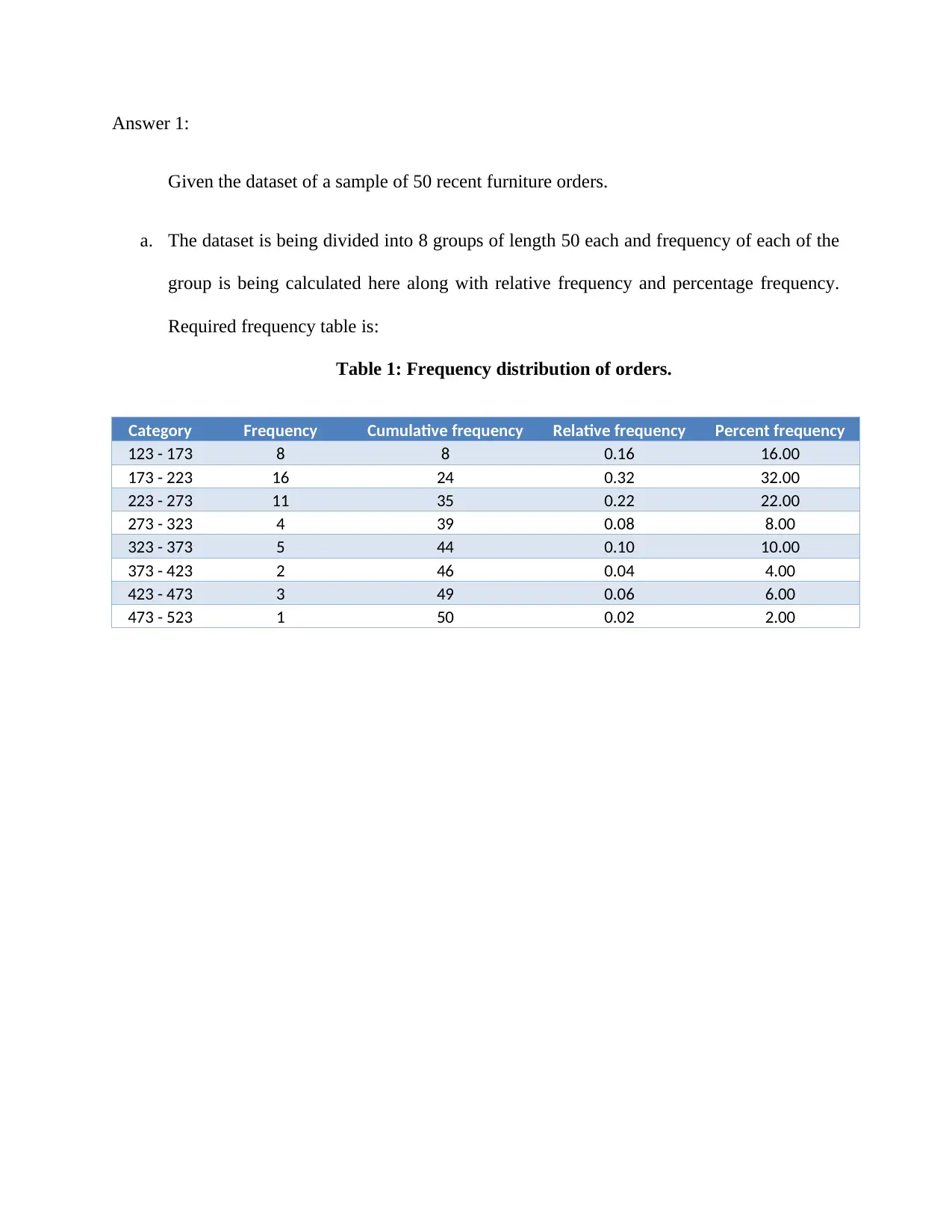
Given the dataset of a sample of 50 recent furniture orders.
a. The dataset is being divided into 8 groups of length 50 each and frequency of each of the
group is being calculated here along with relative frequency and percentage frequency.
Required frequency table is:
Table 1: Frequency distribution of orders.
Category Frequency Cumulative frequency Relative frequency Percent frequency
123 - 173 8 8 0.16 16.00
173 - 223 16 24 0.32 32.00
223 - 273 11 35 0.22 22.00
273 - 323 4 39 0.08 8.00
323 - 373 5 44 0.10 10.00
373 - 423 2 46 0.04 4.00
423 - 473 3 49 0.06 6.00
473 - 523 1 50 0.02 2.00

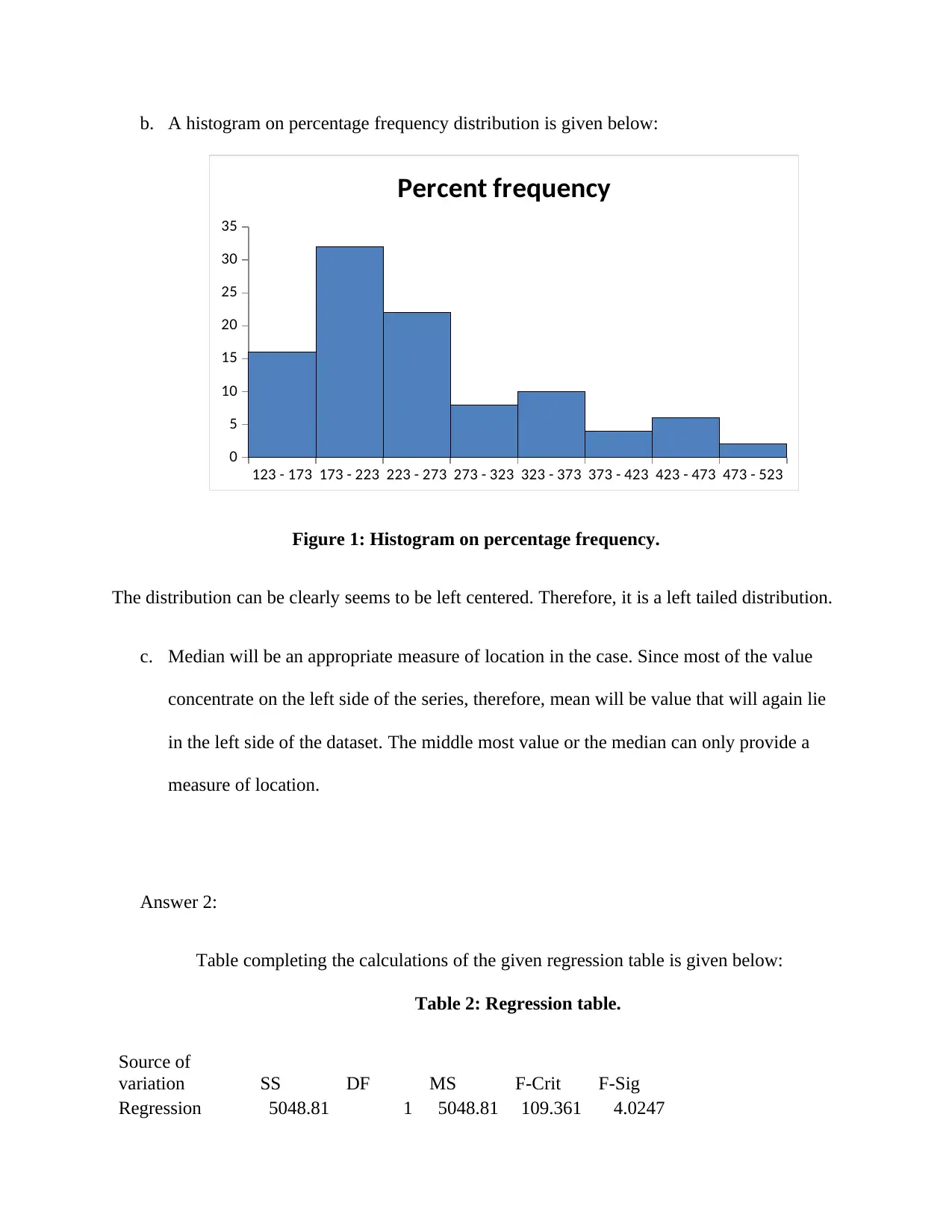
b. A histogram on percentage frequency distribution is given below:
123 - 173 173 - 223 223 - 273 273 - 323 323 - 373 373 - 423 423 - 473 473 - 523
0
5
10
15
20
25
30
35
Percent frequency
Figure 1: Histogram on percentage frequency.
The distribution can be clearly seems to be left centered. Therefore, it is a left tailed distribution.
c. Median will be an appropriate measure of location in the case. Since most of the value
concentrate on the left side of the series, therefore, mean will be value that will again lie
in the left side of the dataset. The middle most value or the median can only provide a
measure of location.
Answer 2:
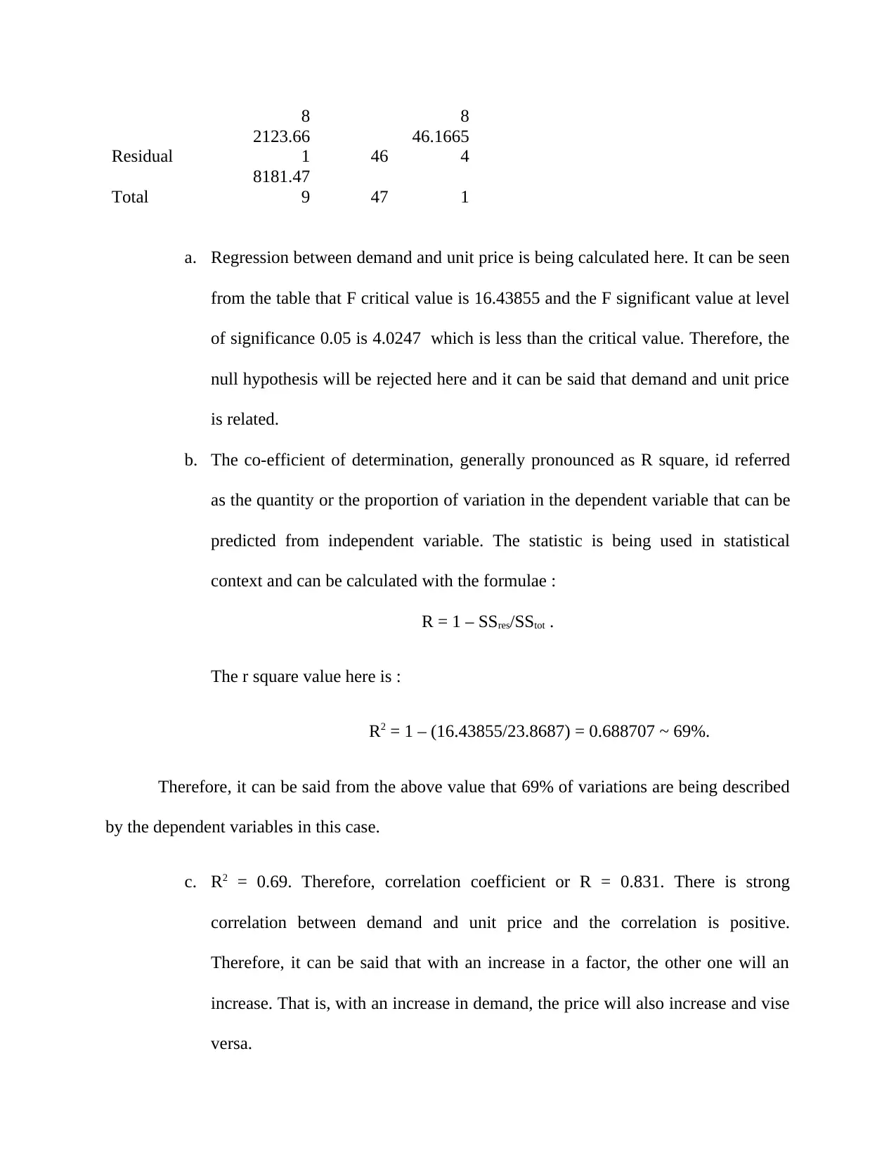
Table completing the calculations of the given regression table is given below:
Table 2: Regression table.
Source of
variation SS DF MS F-Crit F-Sig
Regression 5048.81 1 5048.81 109.361 4.0247

8 8
Residual
2123.66
1 46
46.1665
4
Total
8181.47
9 47 1
a. Regression between demand and unit price is being calculated here. It can be seen
from the table that F critical value is 16.43855 and the F significant value at level
of significance 0.05 is 4.0247 which is less than the critical value. Therefore, the
null hypothesis will be rejected here and it can be said that demand and unit price
is related.
b. The co-efficient of determination, generally pronounced as R square, id referred
as the quantity or the proportion of variation in the dependent variable that can be
predicted from independent variable. The statistic is being used in statistical
context and can be calculated with the formulae :
R = 1 – SSres/SStot .
The r square value here is :
R2 = 1 – (16.43855/23.8687) = 0.688707 ~ 69%.
Therefore, it can be said from the above value that 69% of variations are being described
by the dependent variables in this case.
c. R2 = 0.69. Therefore, correlation coefficient or R = 0.831. There is strong
correlation between demand and unit price and the correlation is positive.
Therefore, it can be said that with an increase in a factor, the other one will an
increase. That is, with an increase in demand, the price will also increase and vise
versa.

Answer 3:
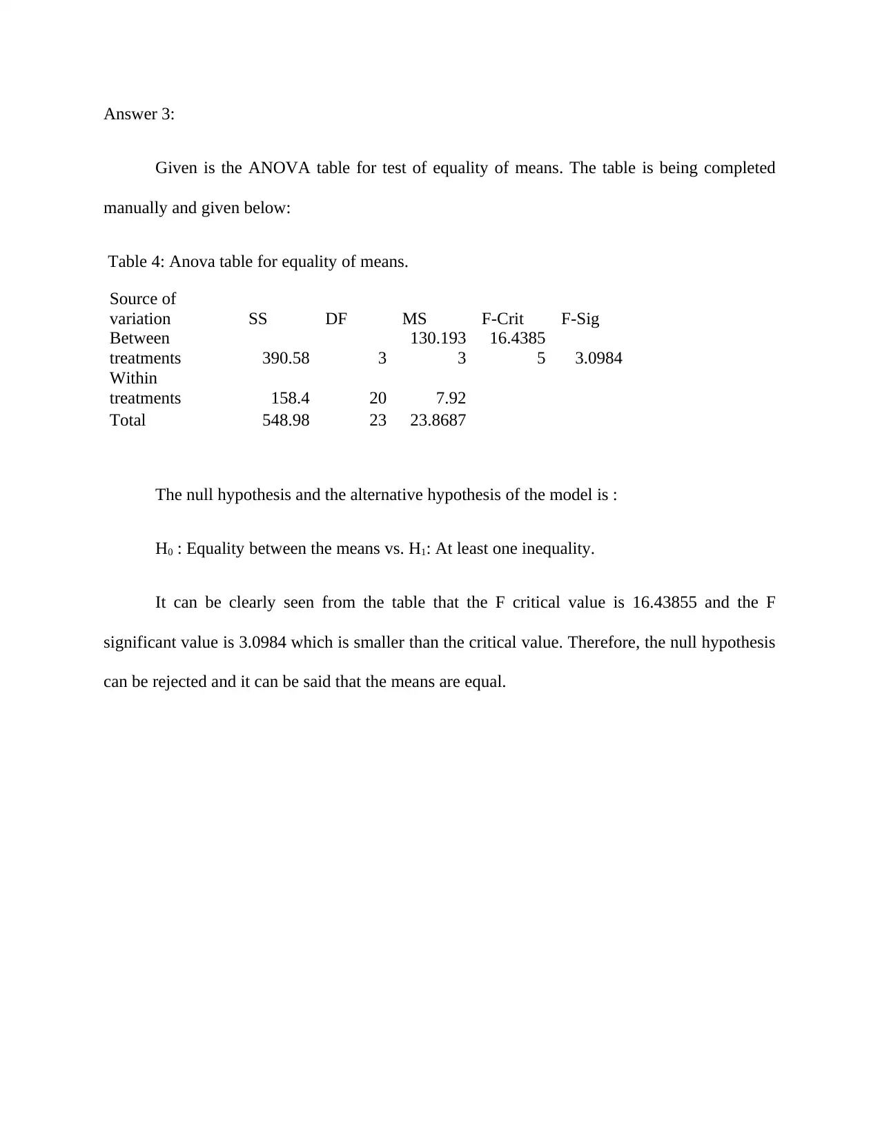
Given is the ANOVA table for test of equality of means. The table is being completed
manually and given below:
Table 4: Anova table for equality of means.
Source of
variation SS DF MS F-Crit F-Sig
Between
treatments 390.58 3
130.193
3
16.4385
5 3.0984
Within
treatments 158.4 20 7.92
Total 548.98 23 23.8687
The null hypothesis and the alternative hypothesis of the model is :
H0 : Equality between the means vs. H1: At least one inequality.
It can be clearly seen from the table that the F critical value is 16.43855 and the F
significant value is 3.0984 which is smaller than the critical value. Therefore, the null hypothesis
can be rejected and it can be said that the means are equal.

Answer 4:
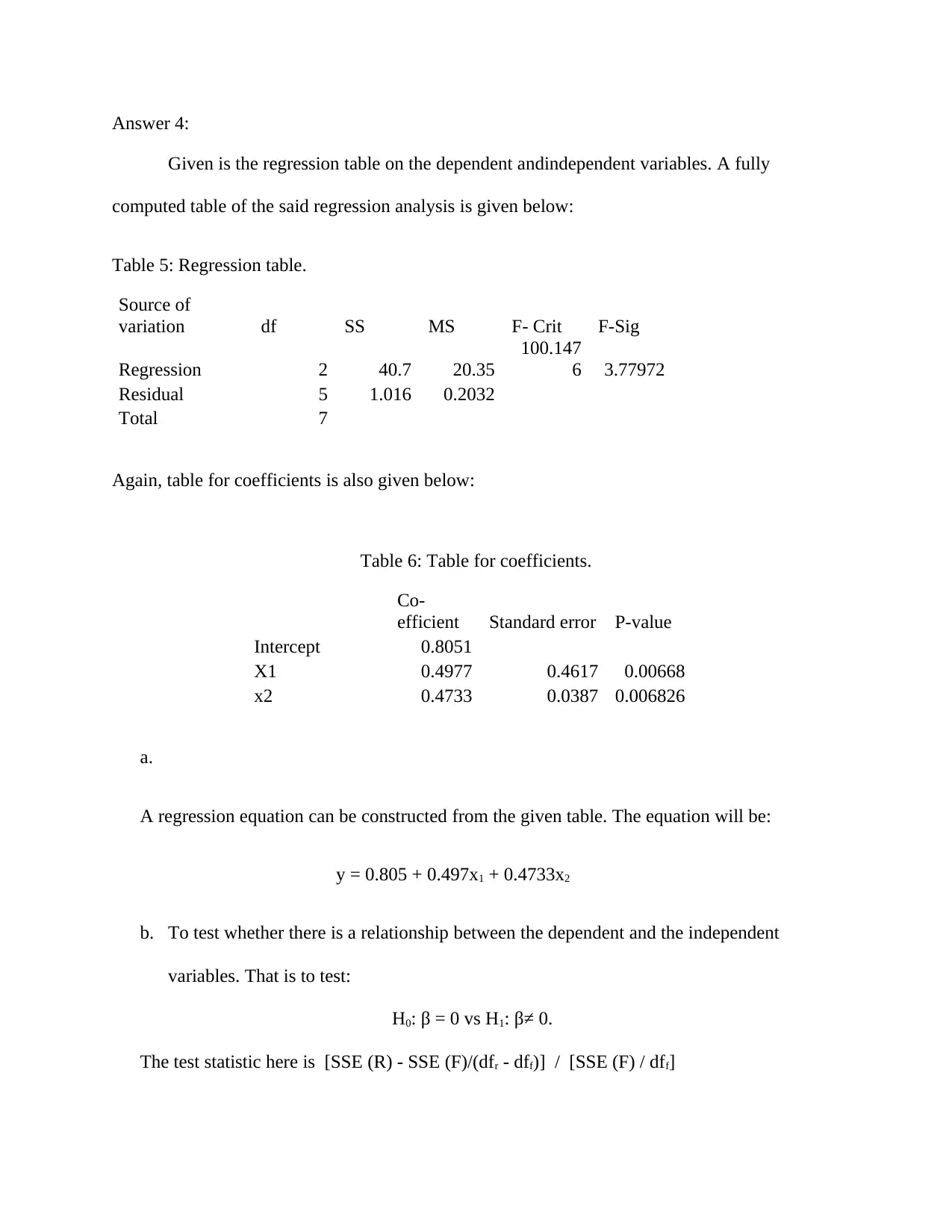
Given is the regression table on the dependent andindependent variables. A fully
computed table of the said regression analysis is given below:
Table 5: Regression table.
Source of
variation df SS MS F- Crit F-Sig
Regression 2 40.7 20.35
100.147
6 3.77972
Residual 5 1.016 0.2032
Total 7
Again, table for coefficients is also given below:
Table 6: Table for coefficients.
Co-
efficient Standard error P-value
Intercept 0.8051
X1 0.4977 0.4617 0.00668
x2 0.4733 0.0387 0.006826
a.
A regression equation can be constructed from the given table. The equation will be:
y = 0.805 + 0.497x1 + 0.4733x2
b. To test whether there is a relationship between the dependent and the independent
variables. That is to test:
H0: β = 0 vs H1: β≠ 0.
The test statistic here is [SSE (R) - SSE (F)/(dfr - dff)] / [SSE (F) / dff]

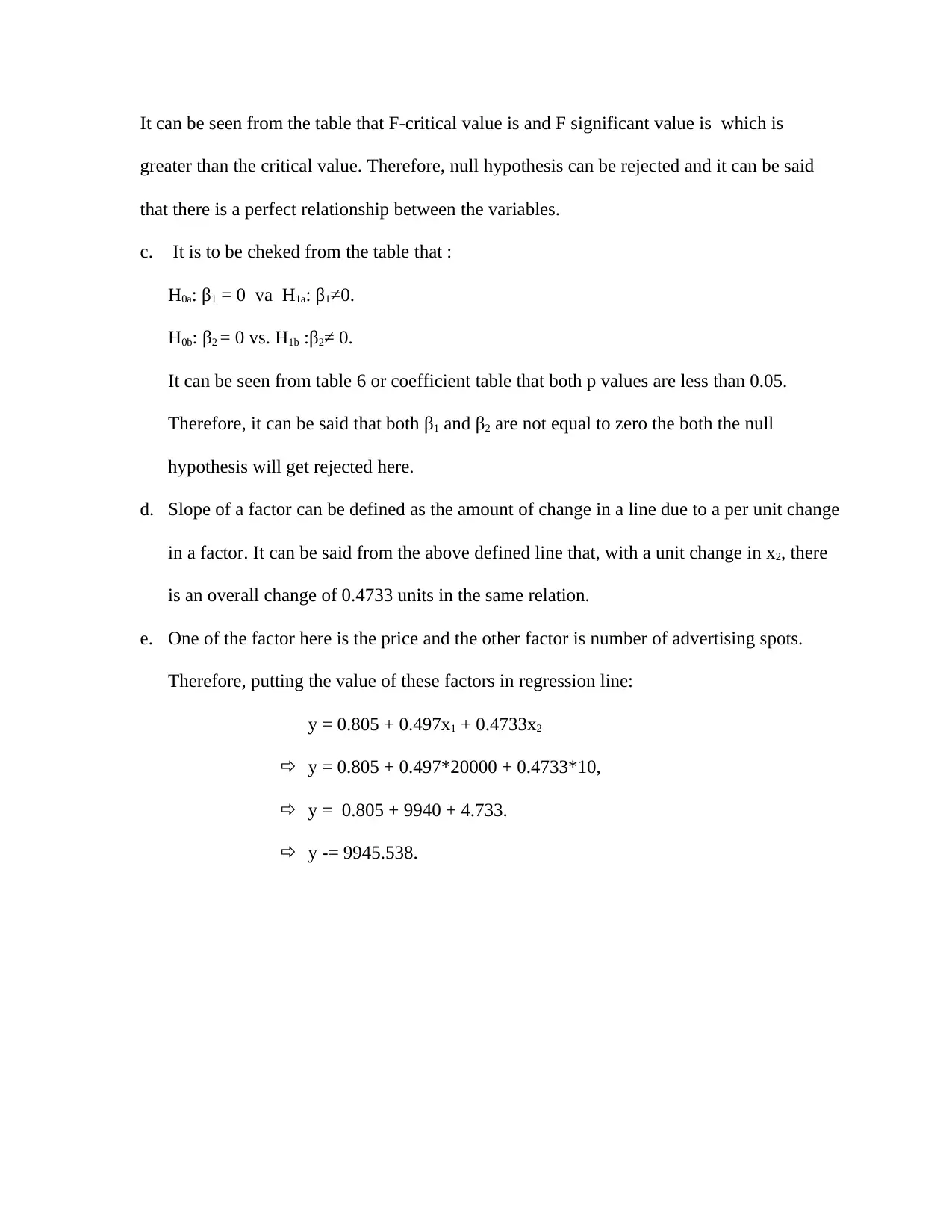
It can be seen from the table that F-critical value is and F significant value is which is
greater than the critical value. Therefore, null hypothesis can be rejected and it can be said
that there is a perfect relationship between the variables.
c. It is to be cheked from the table that :
H0a: β1 = 0 va H1a: β1≠0.
H0b: β2 = 0 vs. H1b :β2≠ 0.
It can be seen from table 6 or coefficient table that both p values are less than 0.05.
Therefore, it can be said that both β1 and β2 are not equal to zero the both the null
hypothesis will get rejected here.
d. Slope of a factor can be defined as the amount of change in a line due to a per unit change
in a factor. It can be said from the above defined line that, with a unit change in x2, there
is an overall change of 0.4733 units in the same relation.
e. One of the factor here is the price and the other factor is number of advertising spots.
Therefore, putting the value of these factors in regression line:
y = 0.805 + 0.497x1 + 0.4733x2
 y = 0.805 + 0.497*20000 + 0.4733*10,
 y = 0.805 + 9940 + 4.733.
 y -= 9945.538.

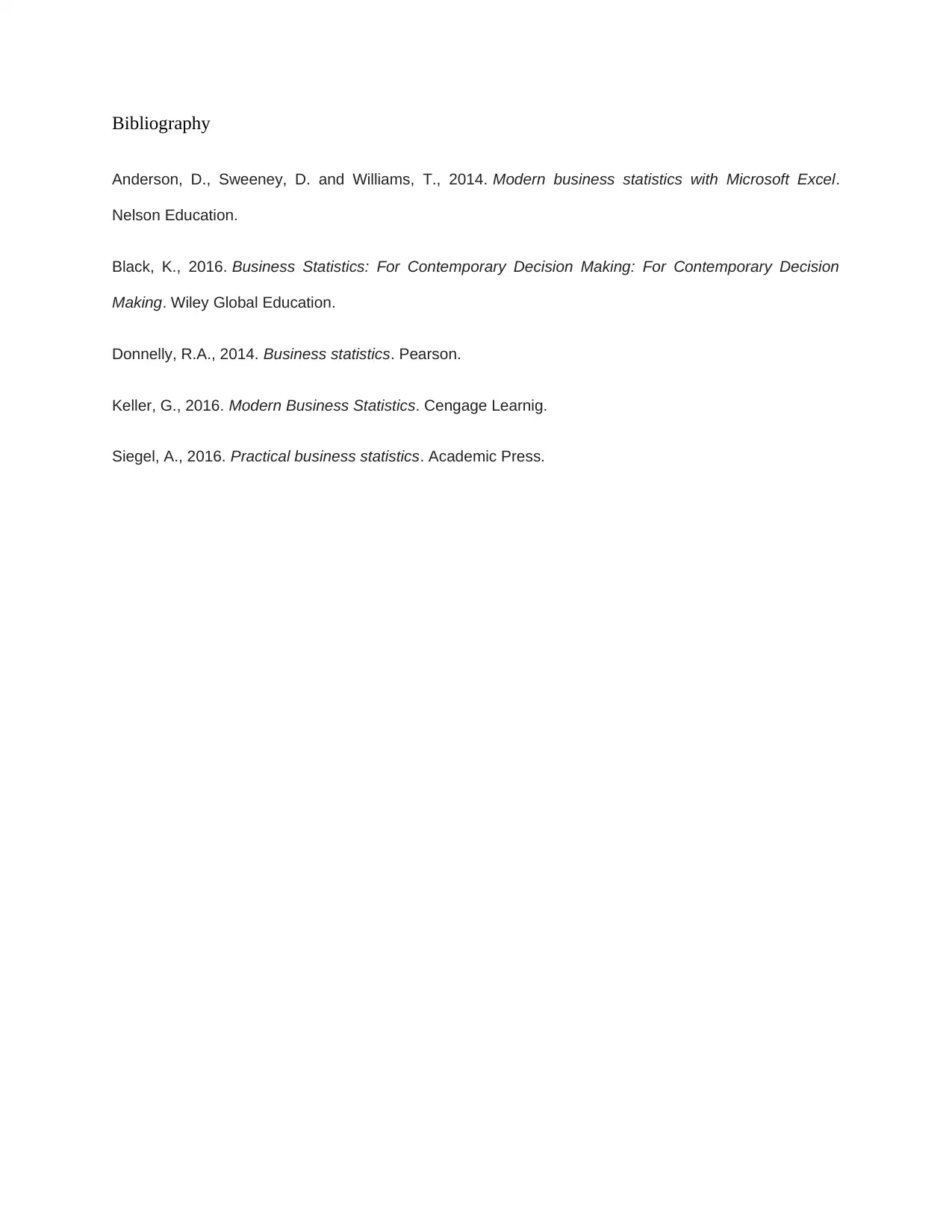
Bibliography
Anderson, D., Sweeney, D. and Williams, T., 2014. Modern business statistics with Microsoft Excel.
Nelson Education.
Black, K., 2016. Business Statistics: For Contemporary Decision Making: For Contemporary Decision
Making. Wiley Global Education.
Donnelly, R.A., 2014. Business statistics. Pearson.
Keller, G., 2016. Modern Business Statistics. Cengage Learnig.
Siegel, A., 2016. Practical business statistics. Academic Press.