Forecasting Sales Techniques

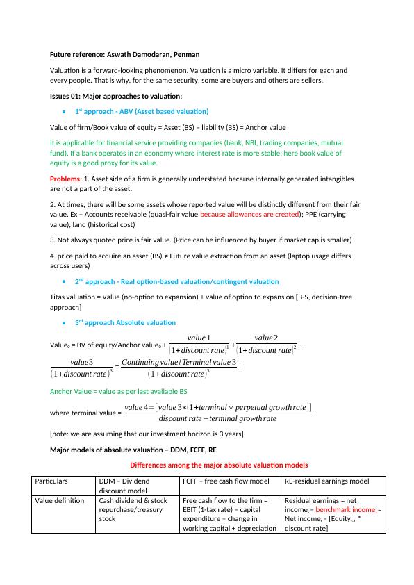
Future reference: Aswath Damodaran, Penman
Valuation is a forward-looking phenomenon. Valuation is a micro variable. It differs for each and
every people. That is why, for the same security, some are buyers and others are sellers.
Issues 01: Major approaches to valuation:
 1st approach - ABV (Asset based valuation)
Value of firm/Book value of equity = Asset (BS) – liability (BS) = Anchor value
It is applicable for financial service providing companies (bank, NBI, trading companies, mutual
fund). If a bank operates in an economy where interest rate is more stable; here book value of
equity is a good proxy for its value.
Problems: 1. Asset side of a firm is generally understated because internally generated intangibles
are not a part of the asset.
2. At times, there will be some assets whose reported value will be distinctly different from their fair
value. Ex – Accounts receivable (quasi-fair value because allowances are created); PPE (carrying
value), land (historical cost)
3. Not always quoted price is fair value. (Price can be influenced by buyer if market cap is smaller)
4. price paid to acquire an asset (BS) ≠ Future value extraction from an asset (laptop usage differs
across users)
 2nd approach - Real option-based valuation/contingent valuation
Titas valuation = Value (no-option to expansion) + value of option to expansion [B-S, decision-tree
approach]
 3rd approach Absolute valuation
Value0 = BV of equity/Anchor value0 + value 1
( 1+ discount rate ) 1 + value 2
( 1+ discount rate )2 +
value3
(1+discount rate)3 + Continuing value/Terminal value 3
(1+ discount rate)3 ;
Anchor Value = value as per last available BS
where terminal value = value 4=[value 3∗( 1+terminal∨ perpetual growthrate ) ]
discount rate−terminal growthrate
[note: we are assuming that our investment horizon is 3 years]
Major models of absolute valuation – DDM, FCFF, RE
Differences among the major absolute valuation models
Particulars DDM – Dividend
discount model
FCFF – free cash flow model RE-residual earnings model
Value definition Cash dividend & stock
repurchase/treasury
stock
Free cash flow to the firm =
EBIT (1-tax rate) – capital
expenditure – change in
working capital + depreciation
Residual earnings = net
incomet – benchmark incomet =
Net incomet – [Equityt-1 *
discount rate]

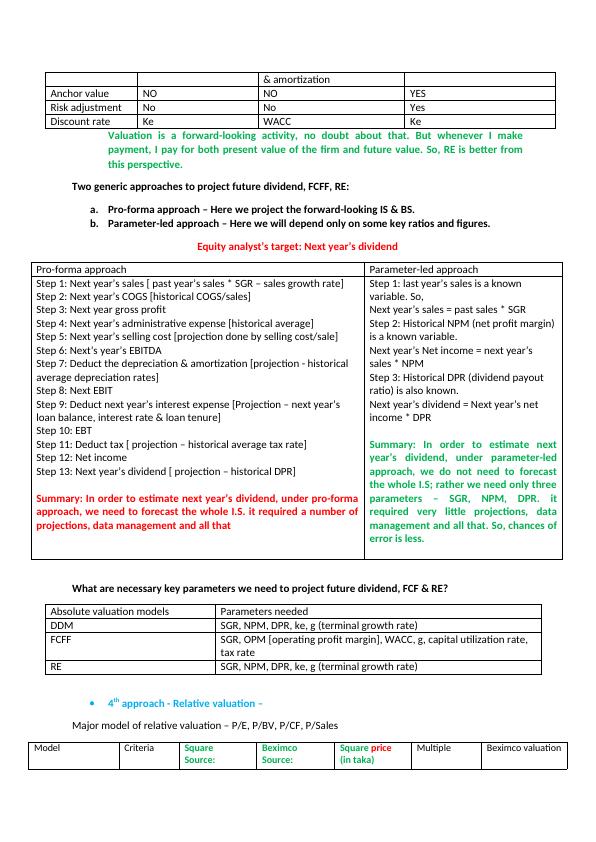
& amortization
Anchor value NO NO YES
Risk adjustment No No Yes
Discount rate Ke WACC Ke
Valuation is a forward-looking activity, no doubt about that. But whenever I make
payment, I pay for both present value of the firm and future value. So, RE is better from
this perspective.
Two generic approaches to project future dividend, FCFF, RE:
a. Pro-forma approach – Here we project the forward-looking IS & BS.
b. Parameter-led approach – Here we will depend only on some key ratios and figures.
Equity analyst’s target: Next year’s dividend
Pro-forma approach Parameter-led approach
Step 1: Next year’s sales [ past year’s sales * SGR – sales growth rate]
Step 2: Next year’s COGS [historical COGS/sales]
Step 3: Next year gross profit
Step 4: Next year’s administrative expense [historical average]
Step 5: Next year’s selling cost [projection done by selling cost/sale]
Step 6: Next’s year’s EBITDA
Step 7: Deduct the depreciation & amortization [projection - historical
average depreciation rates]
Step 8: Next EBIT
Step 9: Deduct next year’s interest expense [Projection – next year’s
loan balance, interest rate & loan tenure]
Step 10: EBT
Step 11: Deduct tax [ projection – historical average tax rate]
Step 12: Net income
Step 13: Next year’s dividend [ projection – historical DPR]
Summary: In order to estimate next year’s dividend, under pro-forma
approach, we need to forecast the whole I.S. it required a number of
projections, data management and all that
Step 1: last year’s sales is a known
variable. So,
Next year’s sales = past sales * SGR
Step 2: Historical NPM (net profit margin)
is a known variable.
Next year’s Net income = next year’s
sales * NPM
Step 3: Historical DPR (dividend payout
ratio) is also known.
Next year’s dividend = Next year’s net
income * DPR
Summary: In order to estimate next
year’s dividend, under parameter-led
approach, we do not need to forecast
the whole I.S; rather we need only three
parameters – SGR, NPM, DPR. it
required very little projections, data
management and all that. So, chances of
error is less.
What are necessary key parameters we need to project future dividend, FCF & RE?
Absolute valuation models Parameters needed
DDM SGR, NPM, DPR, ke, g (terminal growth rate)
FCFF SGR, OPM [operating profit margin], WACC, g, capital utilization rate,
tax rate
RE SGR, NPM, DPR, ke, g (terminal growth rate)
 4th approach - Relative valuation –
Major model of relative valuation – P/E, P/BV, P/CF, P/Sales
Model Criteria Square
Source:
Beximco
Source:
Square price
(in taka)
Multiple Beximco valuation