Linear Programming Model for Gasoline Production

Use Desklib's linear programming model to optimize gasoline production quantities while meeting minimum demand requirements for octane rating and sulfur content. The model takes into account production costs, supervision requirements, and purchase prices for octane rating and sulfur content.

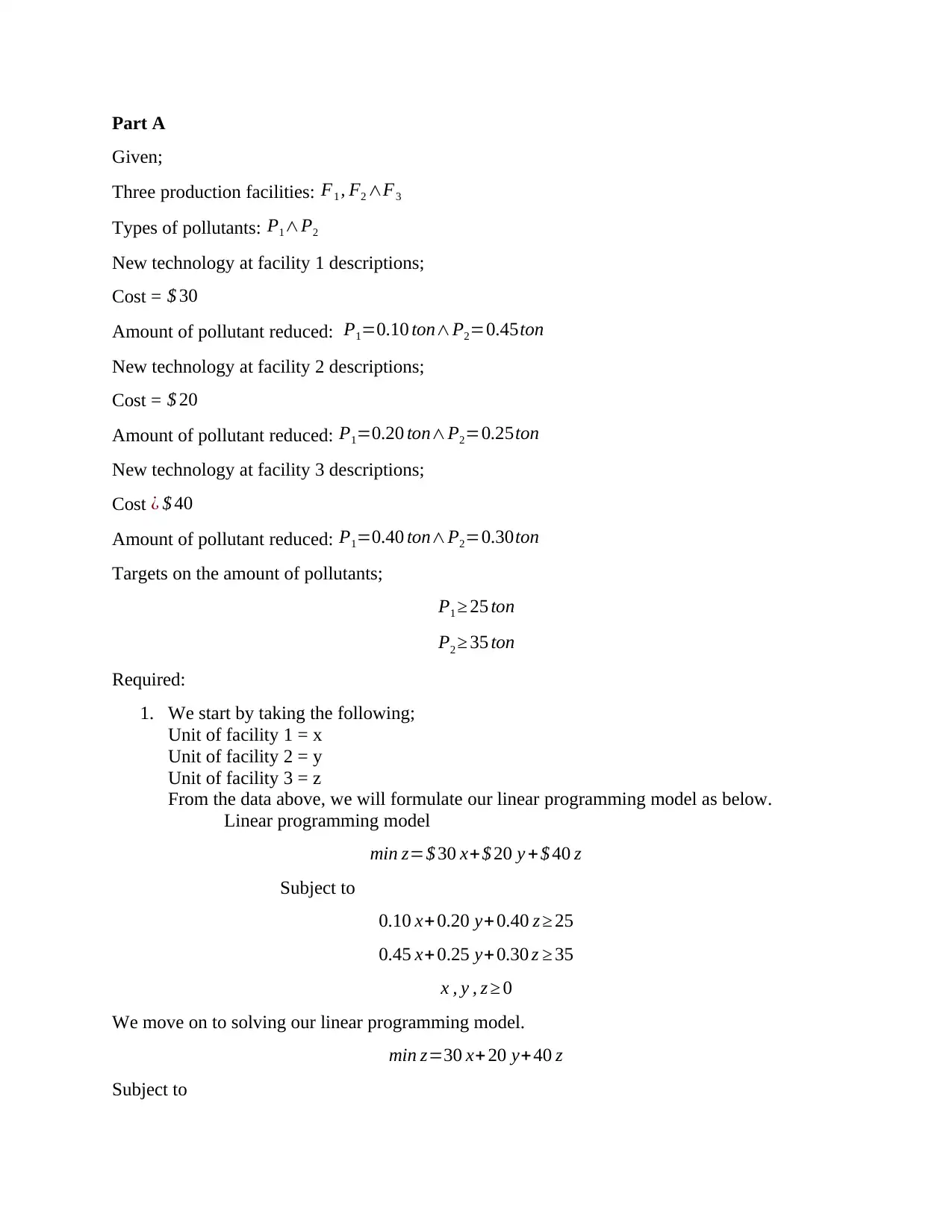
Part A
Given;
Three production facilities: F1 , F2 ∧F3
Types of pollutants: P1∧P2
New technology at facility 1 descriptions;
Cost = $ 30
Amount of pollutant reduced: P1=0.10 ton∧P2=0.45ton
New technology at facility 2 descriptions;
Cost = $ 20
Amount of pollutant reduced: P1=0.20 ton∧P2=0.25ton
New technology at facility 3 descriptions;
Cost ¿ $ 40
Amount of pollutant reduced: P1=0.40 ton∧P2=0.30ton
Targets on the amount of pollutants;
P1 ≥ 25 ton
P2 ≥ 35 ton
Required:
1. We start by taking the following;
Unit of facility 1 = x
Unit of facility 2 = y
Unit of facility 3 = z
From the data above, we will formulate our linear programming model as below.
Linear programming model
min z=$ 30 x+ $ 20 y + $ 40 z
Subject to
0.10 x+ 0.20 y+ 0.40 z ≥ 25
0.45 x+ 0.25 y+ 0.30 z ≥ 35
x , y , z ≥ 0
We move on to solving our linear programming model.
min z=30 x+ 20 y+ 40 z
Subject to

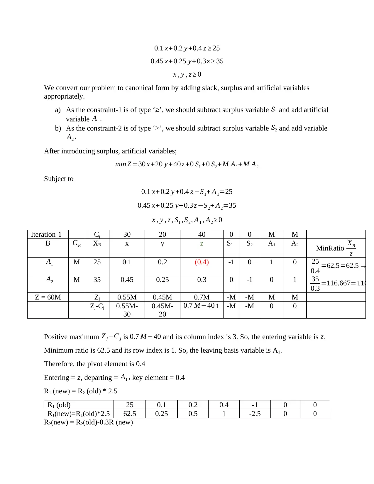
0.1 x+0.2 y +0.4 z ≥ 25
0.45 x+0.25 y+ 0.3 z ≥ 35
x , y , z ≥ 0
We convert our problem to canonical form by adding slack, surplus and artificial variables
appropriately.
a) As the constraint-1 is of type ‘ ≥’, we should subtract surplus variable S1 and add artificial
variable A1 .
b) As the constraint-2 is of type ‘ ≥’, we should subtract surplus variable S2 and add variable
A2 .
After introducing surplus, artificial variables;
min Z =30 x +20 y +40 z +0 S1 +0 S2 + M A1+ M A2
Subject to
0.1 x+0.2 y +0.4 z −S1+ A1=25
0.45 x+0.25 y+ 0.3 z −S2+ A2=35
x , y , z , S1 , S2 , A1 , A2 ≥ 0
Iteration-1 Cj 30 20 40 0 0 M M
B CB XB x y z S1 S2 A1 A2 MinRatio XB
z
A1 M 25 0.1 0.2 (0.4) -1 0 1 0 25
0.4 =62.5=62.5 →
A2 M 35 0.45 0.25 0.3 0 -1 0 1 35
0.3 =116.667=116.66
Z = 60M Zj 0.55M 0.45M 0.7M -M -M M M
Zj-Cj 0.55M-
30
0.45M-
20
0.7 M−40 ↑ -M -M 0 0
Positive maximum Z j−C j is 0.7 M−40 and its column index is 3. So, the entering variable is z.
Minimum ratio is 62.5 and its row index is 1. So, the leaving basis variable is A1.
Therefore, the pivot element is 0.4
Entering = z, departing = A1 , key element = 0.4
R1 (new) = R2 (old) * 2.5
R1 (old) 25 0.1 0.2 0.4 -1 0 0
R1(new)=R1(old)*2.5 62.5 0.25 0.5 1 -2.5 0 0
R2(new) = R2(old)-0.3R1(new)

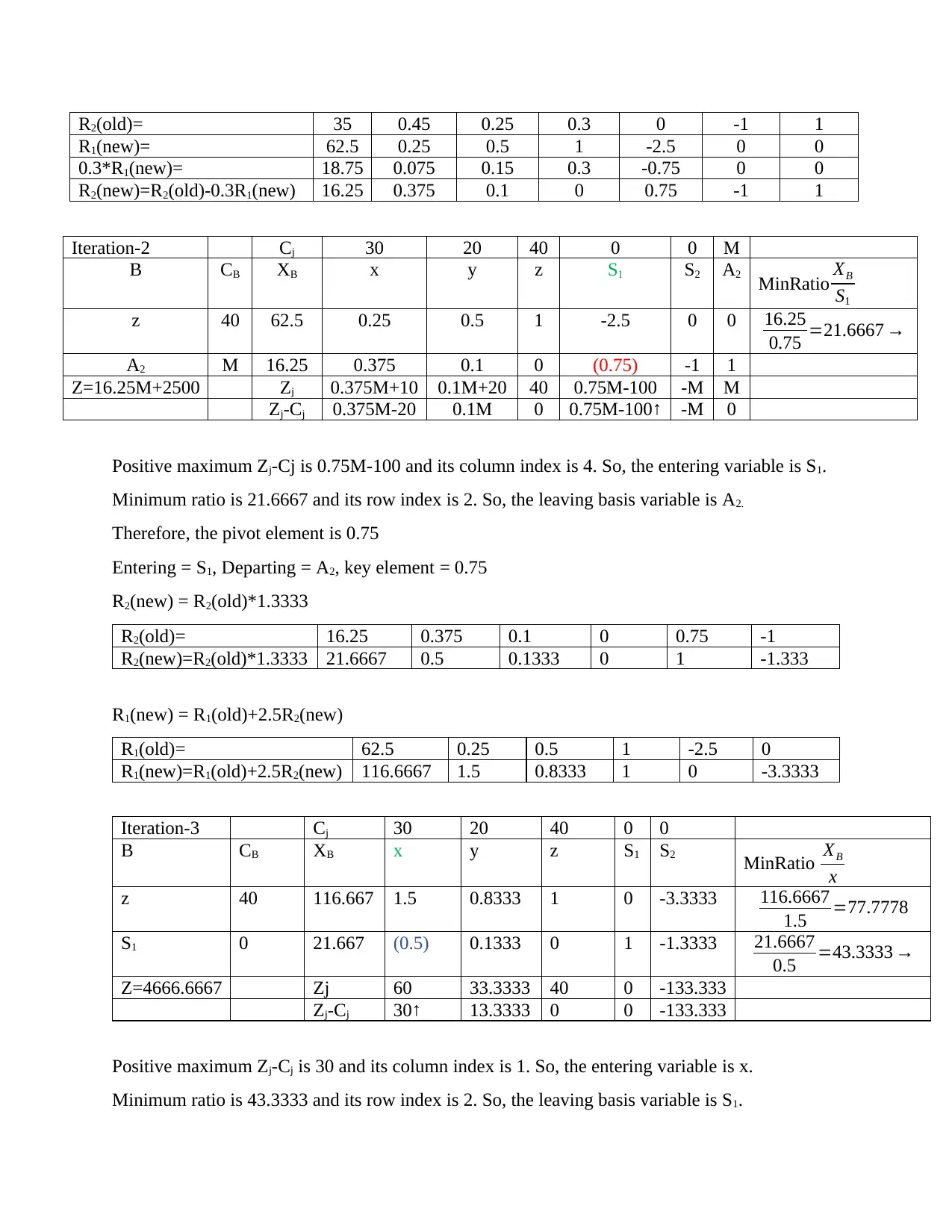
R2(old)= 35 0.45 0.25 0.3 0 -1 1
R1(new)= 62.5 0.25 0.5 1 -2.5 0 0
0.3*R1(new)= 18.75 0.075 0.15 0.3 -0.75 0 0
R2(new)=R2(old)-0.3R1(new) 16.25 0.375 0.1 0 0.75 -1 1
Iteration-2 Cj 30 20 40 0 0 M
B CB XB x y z S1 S2 A2
MinRatio XB
S1
z 40 62.5 0.25 0.5 1 -2.5 0 0 16.25
0.75 =21.6667 →
A2 M 16.25 0.375 0.1 0 (0.75) -1 1
Z=16.25M+2500 Zj 0.375M+10 0.1M+20 40 0.75M-100 -M M
Zj-Cj 0.375M-20 0.1M 0 0.75M-100 ↑ -M 0
Positive maximum Zj-Cj is 0.75M-100 and its column index is 4. So, the entering variable is S1.
Minimum ratio is 21.6667 and its row index is 2. So, the leaving basis variable is A2.
Therefore, the pivot element is 0.75
Entering = S1, Departing = A2, key element = 0.75
R2(new) = R2(old)*1.3333
R2(old)= 16.25 0.375 0.1 0 0.75 -1
R2(new)=R2(old)*1.3333 21.6667 0.5 0.1333 0 1 -1.333
R1(new) = R1(old)+2.5R2(new)
R1(old)= 62.5 0.25 0.5 1 -2.5 0
R1(new)=R1(old)+2.5R2(new) 116.6667 1.5 0.8333 1 0 -3.3333
Iteration-3 Cj 30 20 40 0 0
B CB XB x y z S1 S2 MinRatio XB
x
z 40 116.667 1.5 0.8333 1 0 -3.3333 116.6667
1.5 =77.7778
S1 0 21.667 (0.5) 0.1333 0 1 -1.3333 21.6667
0.5 =43.3333 →
Z=4666.6667 Zj 60 33.3333 40 0 -133.333
Zj-Cj 30↑ 13.3333 0 0 -133.333
Positive maximum Zj-Cj is 30 and its column index is 1. So, the entering variable is x.
Minimum ratio is 43.3333 and its row index is 2. So, the leaving basis variable is S1.

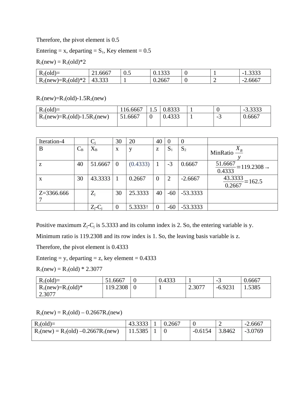
Therefore, the pivot element is 0.5
Entering = x, departing = S1, Key element = 0.5
R2(new) = R2(old)*2
R2(old)= 21.6667 0.5 0.1333 0 1 -1.3333
R2(new)=R2(old)*2 43.333 1 0.2667 0 2 -2.6667
R1(new)=R1(old)-1.5R2(new)
R1(old)= 116.6667 1.5 0.8333 1 0 -3.3333
R1(new)=R1(old)-1.5R2(new) 51.6667 0 0.4333 1 -3 0.6667
Iteration-4 Cj 30 20 40 0 0
B CB XB x y z S1 S2 MinRatio XB
y
z 40 51.6667 0 (0.4333) 1 -3 0.6667 51.6667
0.4333 =119.2308→
x 30 43.3333 1 0.2667 0 2 -2.6667 43.3333
0.2667 =162.5
Z=3366.666
7
Zj 30 25.3333 40 -60 -53.3333
Zj-Cj 0 5.3333↑ 0 -60 -53.3333
Positive maximum Zj-Cj is 5.3333 and its column index is 2. So, the entering variable is y.
Minimum ratio is 119.2308 and its row index is 1. So, the leaving basis variable is z.
Therefore, the pivot element is 0.4333
Entering = y, departing = z, key element = 0.4333
R1(new) = R1(old) * 2.3077
R1(old)= 51.6667 0 0.4333 1 -3 0.6667
R1(new)=R1(old)*
2.3077
119.2308 0 1 2.3077 -6.9231 1.5385
R2(new) = R2(old) – 0.2667R1(new)
R2(old)= 43.3333 1 0.2667 0 2 -2.6667
R2(new) = R2(old) –0.2667R1(new) 11.5385 1 0 -0.6154 3.8462 -3.0769

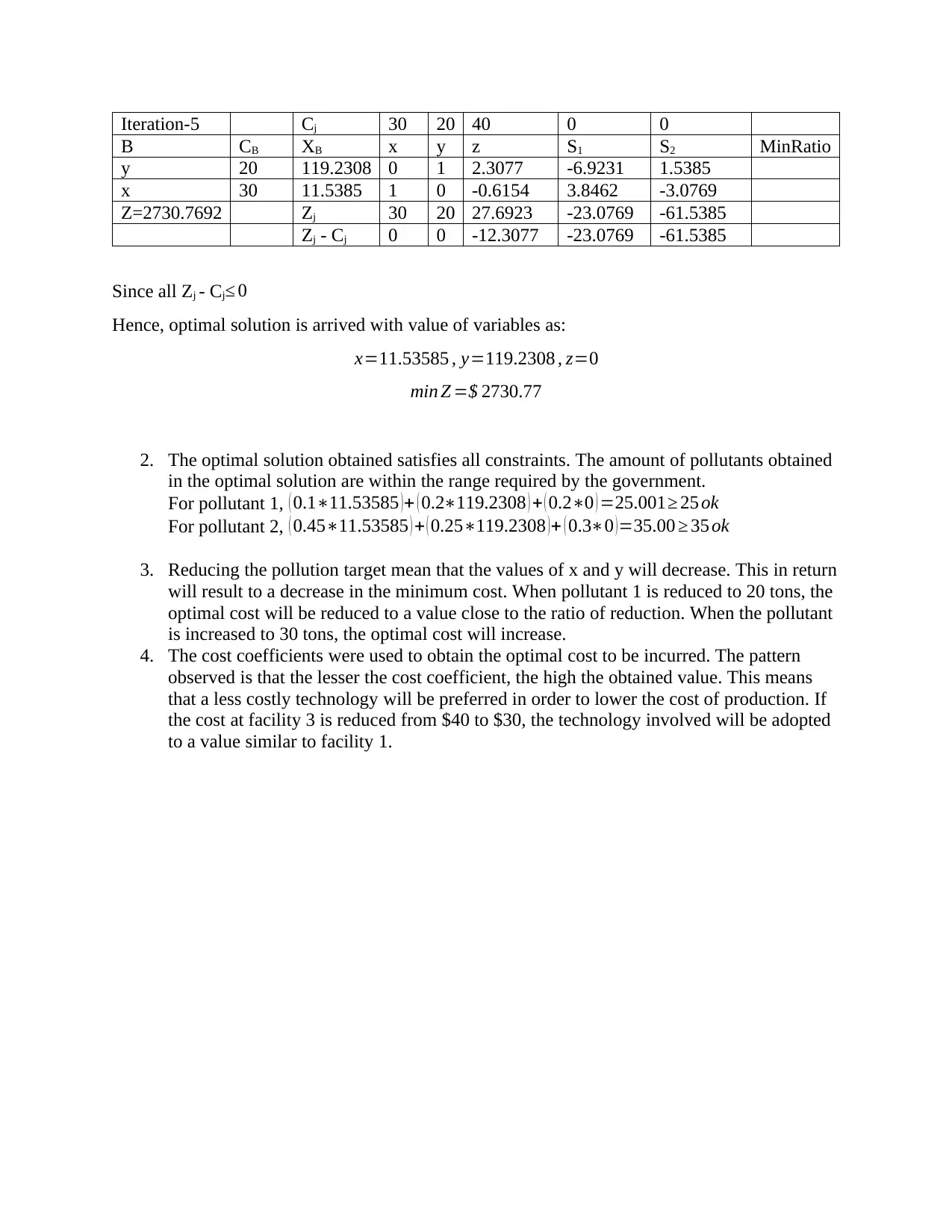
Iteration-5 Cj 30 20 40 0 0
B CB XB x y z S1 S2 MinRatio
y 20 119.2308 0 1 2.3077 -6.9231 1.5385
x 30 11.5385 1 0 -0.6154 3.8462 -3.0769
Z=2730.7692 Zj 30 20 27.6923 -23.0769 -61.5385
Zj - Cj 0 0 -12.3077 -23.0769 -61.5385
Since all Zj - Cj≤ 0
Hence, optimal solution is arrived with value of variables as:
x=11.53585 , y=119.2308 , z=0
min Z =$ 2730.77
2. The optimal solution obtained satisfies all constraints. The amount of pollutants obtained
in the optimal solution are within the range required by the government.
For pollutant 1, ( 0.1∗11.53585 ) + ( 0.2∗119.2308 ) + ( 0.2∗0 ) =25.001≥ 25 ok
For pollutant 2, ( 0.45∗11.53585 ) + ( 0.25∗119.2308 ) + ( 0.3∗0 ) =35.00 ≥ 35 ok
3. Reducing the pollution target mean that the values of x and y will decrease. This in return
will result to a decrease in the minimum cost. When pollutant 1 is reduced to 20 tons, the
optimal cost will be reduced to a value close to the ratio of reduction. When the pollutant
is increased to 30 tons, the optimal cost will increase.
4. The cost coefficients were used to obtain the optimal cost to be incurred. The pattern
observed is that the lesser the cost coefficient, the high the obtained value. This means
that a less costly technology will be preferred in order to lower the cost of production. If
the cost at facility 3 is reduced from $40 to $30, the technology involved will be adopted
to a value similar to facility 1.

Part B
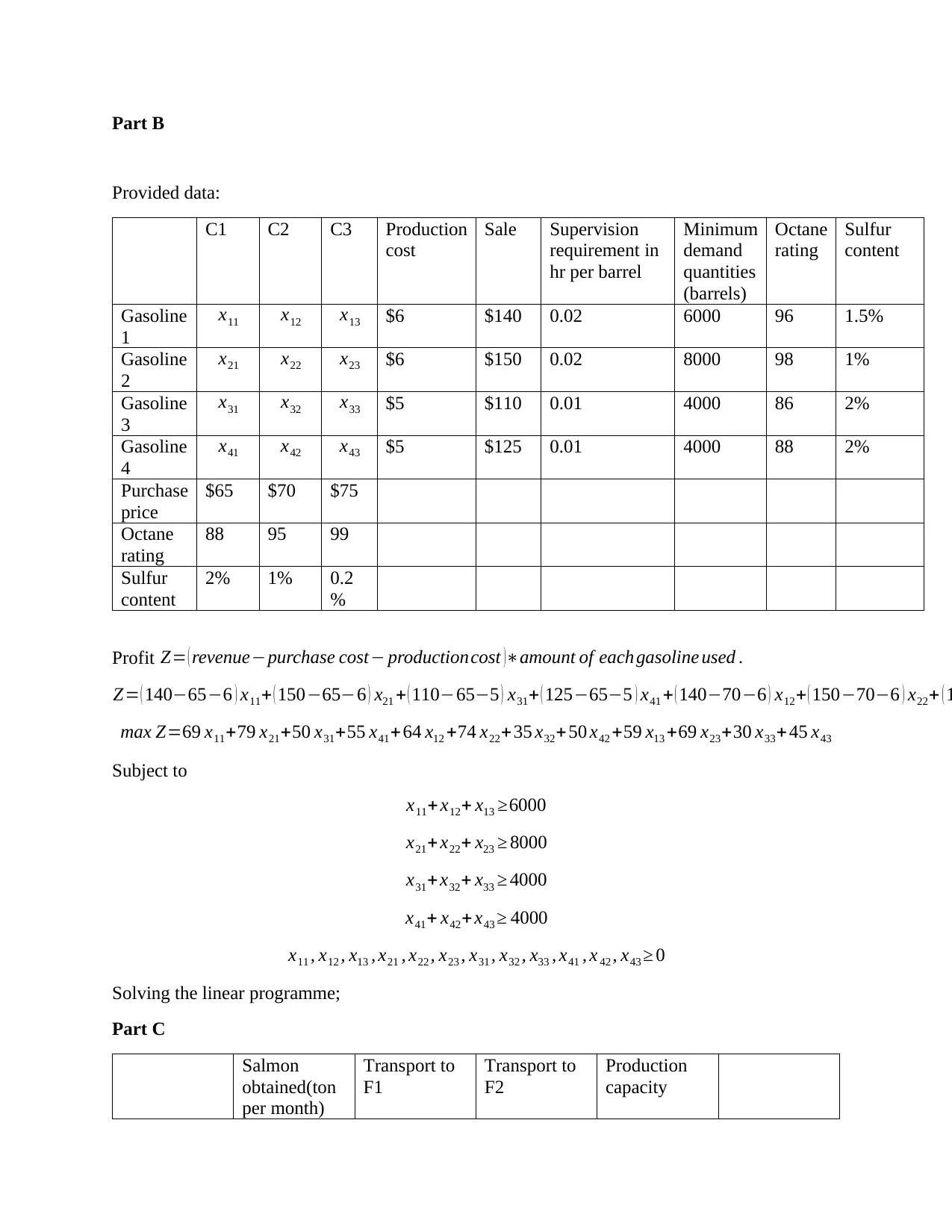
Provided data:
C1 C2 C3 Production
cost
Sale Supervision
requirement in
hr per barrel
Minimum
demand
quantities
(barrels)
Octane
rating
Sulfur
content
Gasoline
1
x11 x12 x13 $6 $140 0.02 6000 96 1.5%
Gasoline
2
x21 x22 x23 $6 $150 0.02 8000 98 1%
Gasoline
3
x31 x32 x33 $5 $110 0.01 4000 86 2%
Gasoline
4
x41 x42 x43 $5 $125 0.01 4000 88 2%
Purchase
price
$65 $70 $75
Octane
rating
88 95 99
Sulfur
content
2% 1% 0.2
%
Profit Z= ( revenue−purchase cost− productioncost )∗amount of each gasoline used .
Z= ( 140−65−6 ) x11+ ( 150−65−6 ) x21 + ( 110−65−5 ) x31+ ( 125−65−5 ) x41 + ( 140−70−6 ) x12+ ( 150−70−6 ) x22+ ( 1
max Z=69 x11+79 x21+50 x31+55 x41+64 x12 +74 x22+ 35 x32+50 x42 +59 x13 +69 x23+30 x33+ 45 x43
Subject to
x11+ x12+ x13 ≥6000
x21+ x22+ x23 ≥ 8000
x31+ x32+ x33 ≥ 4000
x41+ x42+ x43 ≥ 4000
x11 , x12 , x13 , x21 , x22 , x23 , x31 , x32 , x33 , x41 , x 42 , x43 ≥ 0
Solving the linear programme;
Part C
Salmon
obtained(ton
per month)
Transport to
F1
Transport to
F2
Production
capacity

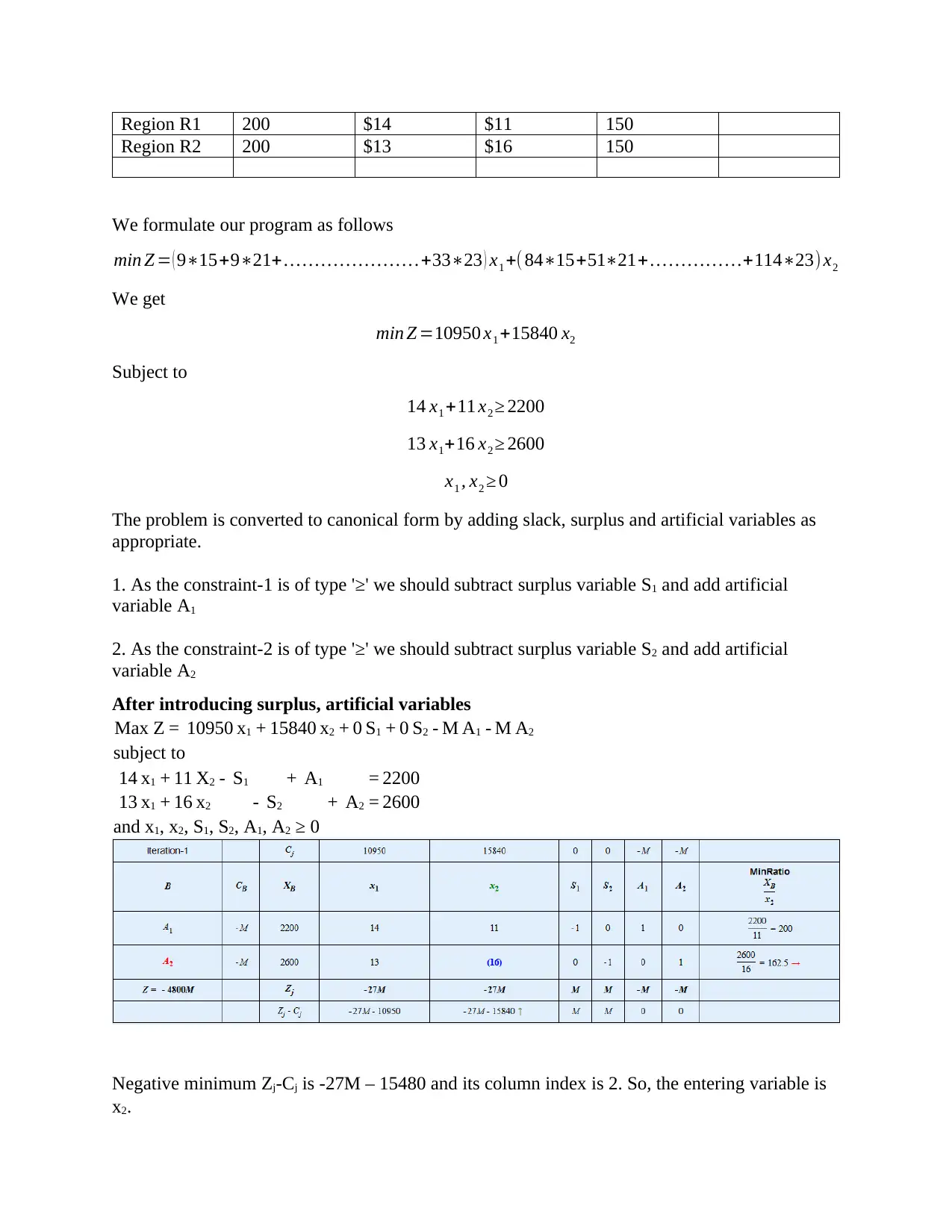
Region R1 200 $14 $11 150
Region R2 200 $13 $16 150
We formulate our program as follows
min Z = ( 9∗15+9∗21+ … … … … … … … .+33∗23 ) x1 +( 84∗15+51∗21+ … … … … …+114∗23) x2
We get
min Z =10950 x1 +15840 x2
Subject to
14 x1 +11 x2 ≥ 2200
13 x1+16 x2 ≥ 2600
x1 , x2 ≥ 0
The problem is converted to canonical form by adding slack, surplus and artificial variables as
appropriate.
1. As the constraint-1 is of type '≥' we should subtract surplus variable S1 and add artificial
variable A1
2. As the constraint-2 is of type '≥' we should subtract surplus variable S2 and add artificial
variable A2
After introducing surplus, artificial variables
Max Z = 10950 x1 + 15840 x2 + 0 S1 + 0 S2 - M A1 - M A2
subject to
14 x1 + 11 X2 - S1 + A1 = 2200
13 x1 + 16 x2 - S2 + A2 = 2600
and x1, x2, S1, S2, A1, A2 ≥ 0
Negative minimum Zj-Cj is -27M – 15480 and its column index is 2. So, the entering variable is
x2.

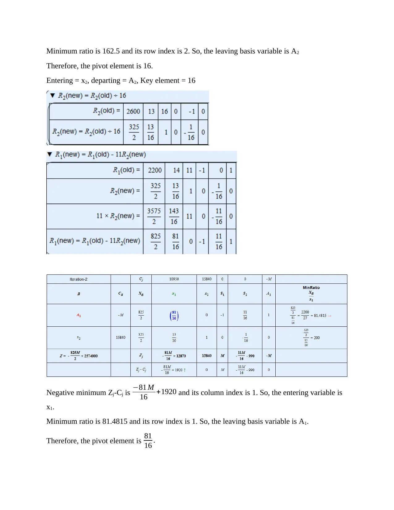
Minimum ratio is 162.5 and its row index is 2. So, the leaving basis variable is A2
Therefore, the pivot element is 16.
Entering = x2, departing = A2, Key element = 16
Negative minimum Zj-Cj is −81 M
16 +1920 and its column index is 1. So, the entering variable is
x1.
Minimum ratio is 81.4815 and its row index is 1. So, the leaving basis variable is A1.
Therefore, the pivot element is 81
16 .

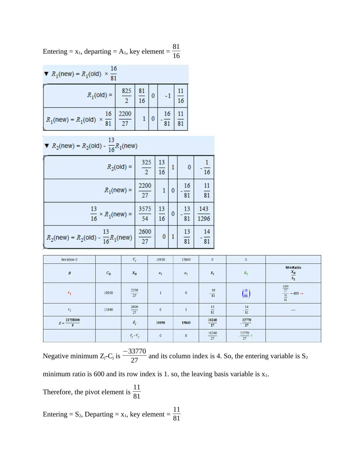
Entering = x1, departing = A1, key element = 81
16
Negative minimum Zj-Cj is −33770
27 and its column index is 4. So, the entering variable is S2
minimum ratio is 600 and its row index is 1. so, the leaving basis variable is x1.
Therefore, the pivot element is 11
81
Entering = S2, Departing = x1, key element = 11
81

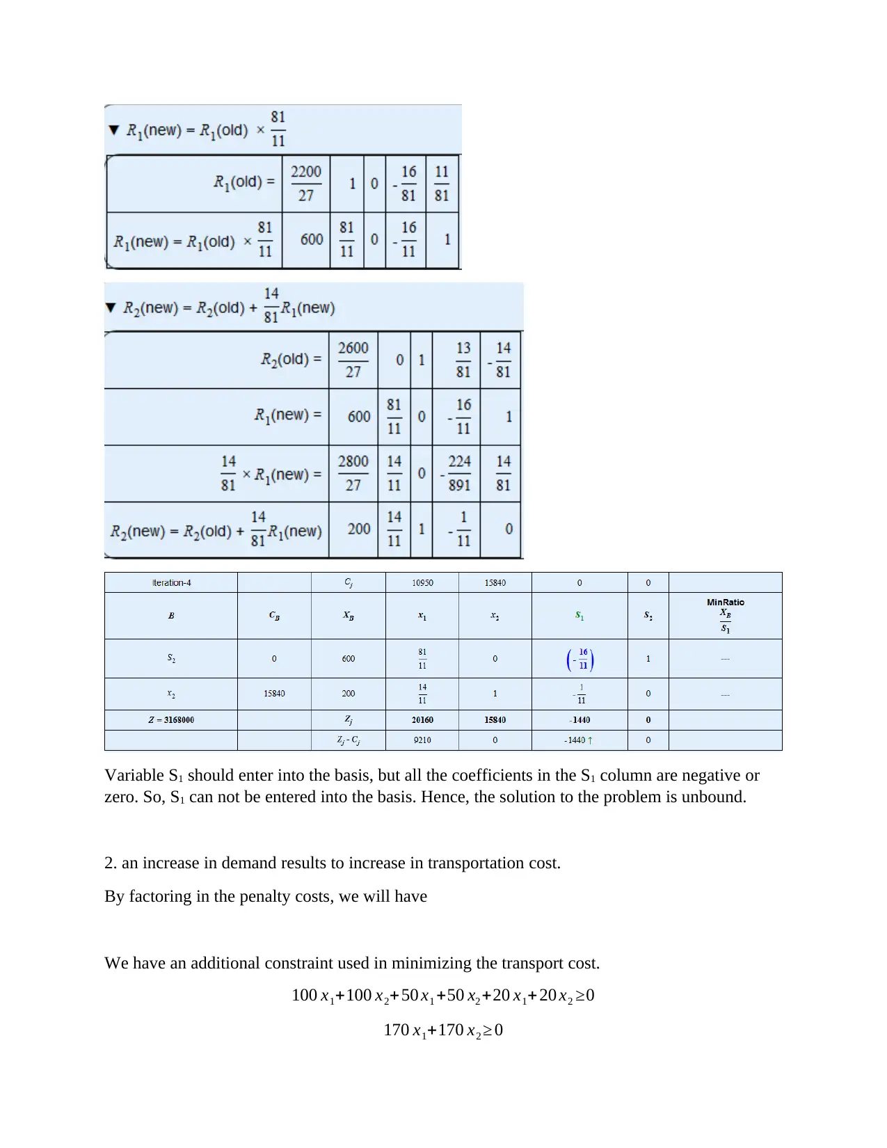
Variable S1 should enter into the basis, but all the coefficients in the S1 column are negative or
zero. So, S1 can not be entered into the basis. Hence, the solution to the problem is unbound.
2. an increase in demand results to increase in transportation cost.
By factoring in the penalty costs, we will have
We have an additional constraint used in minimizing the transport cost.
100 x1+100 x2+50 x1 +50 x2 +20 x1+ 20 x2 ≥0
170 x1+170 x2 ≥ 0

The solution will be infeasible since the optimal objective value is small.
The demand will not be met since the optimal value will be unrealistic.
Part D
Provided data:
Total pollution before the projects = S units
Set of projects = P
Units of money = y
Time period = t
Interest rate = r%
Money available after t+1 = (1+r)y
Total initial budget = I
Outsource = Bt
Share = f
Total budget = allocated≥ total budget allocated in the previous period
Balance = E
Linear program
min Z =∑ apt x , S
Subject to
T + f +B t ≥ T previously allocated
S+ P ≥ E
T , f , Bt ≥ 0
Part E
Q1

a) The model is infeasible because some constraints are relatively high as compared to other
constraints.
b) The model can be unbounded. Reason behind this is that it is infeasible meaning that
some constraints will not be satisfied.
Q2
a) The model will remain feasible. Since the value of optimal objective value is very high,
the model will still be feasible.
b) The optimal objective value will not remain the same. It will reduce.
Q3. An increase in resources results to an increase in objective goal. Therefore, the objective
goal will be greater than 999.
Q4. Slack variables are tight and bounding when they are zero. Therefore, when the slack is
positive the result become lose and less bounded. The demand satisfaction will then be reduced.

References
Charnes, A. and Cooper, W.W., 1962. Programming with linear fractional functionals. Naval Research
logistics quarterly, 9(3 4), pp.181-186.‐
Karmarkar, N., 1984, December. A new polynomial-time algorithm for linear programming. In
Proceedings of the sixteenth annual ACM symposium on Theory of computing (pp. 302-311). ACM.
Zimmermann, H.J., 1978. Fuzzy programming and linear programming with several objective functions.
Fuzzy sets and systems, 1(1), pp.45-55.
Candes, E.J. and Tao, T., 2005. Decoding by linear programming. IEEE transactions on information theory,
51(12), pp.4203-4215.
Luenberger, D.G., 1973. Introduction to linear and nonlinear programming.
Nash, S.G. and Sofer, A., 1996. Linear and nonlinear programming.