Ask a question from expert
Global stiffness matrix Assignemnt PDF
8 Pages1388 Words206 Views
Added on 2021-06-18
Global stiffness matrix Assignemnt PDF
Added on 2021-06-18
BookmarkShareRelated Documents
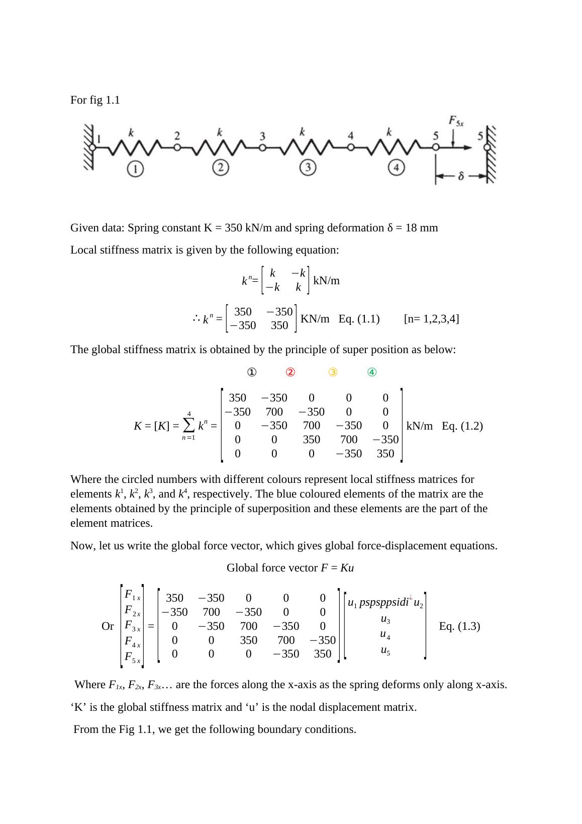
For fig 1.1Given data: Spring constant K = 350 kN/m and spring deformation δ = 18 mmLocal stiffness matrix is given by the following equation:kn= [k−k−kk] kN/m∴kn = [350−350−350350] KN/m Eq. (1.1)[n= 1,2,3,4]The global stiffness matrix is obtained by the principle of super position as below:①②③④K = [K] = ∑n=14kn = [350−350000−350700−350000−350700−350000350700−350000−350350] kN/m Eq. (1.2)Where the circled numbers with different colours represent local stiffness matrices for elements k1, k2, k3, and k4, respectively. The blue coloured elements of the matrix are the elements obtained by the principle of superposition and these elements are the part of the element matrices.Now, let us write the global force vector, which gives global force-displacement equations.Global force vector F = KuOr [F1xF2xF3xF4xF5x] = [350−350000−350700−350000−350700−350000350700−350000−350350][u1pspsppsidi¿u2u3u4u5]Eq. (1.3)Where F1x, F2x, F3x... are the forces along the x-axis as the spring deforms only along x-axis.‘K’ is the global stiffness matrix and ‘u’ is the nodal displacement matrix. From the Fig 1.1, we get the following boundary conditions.
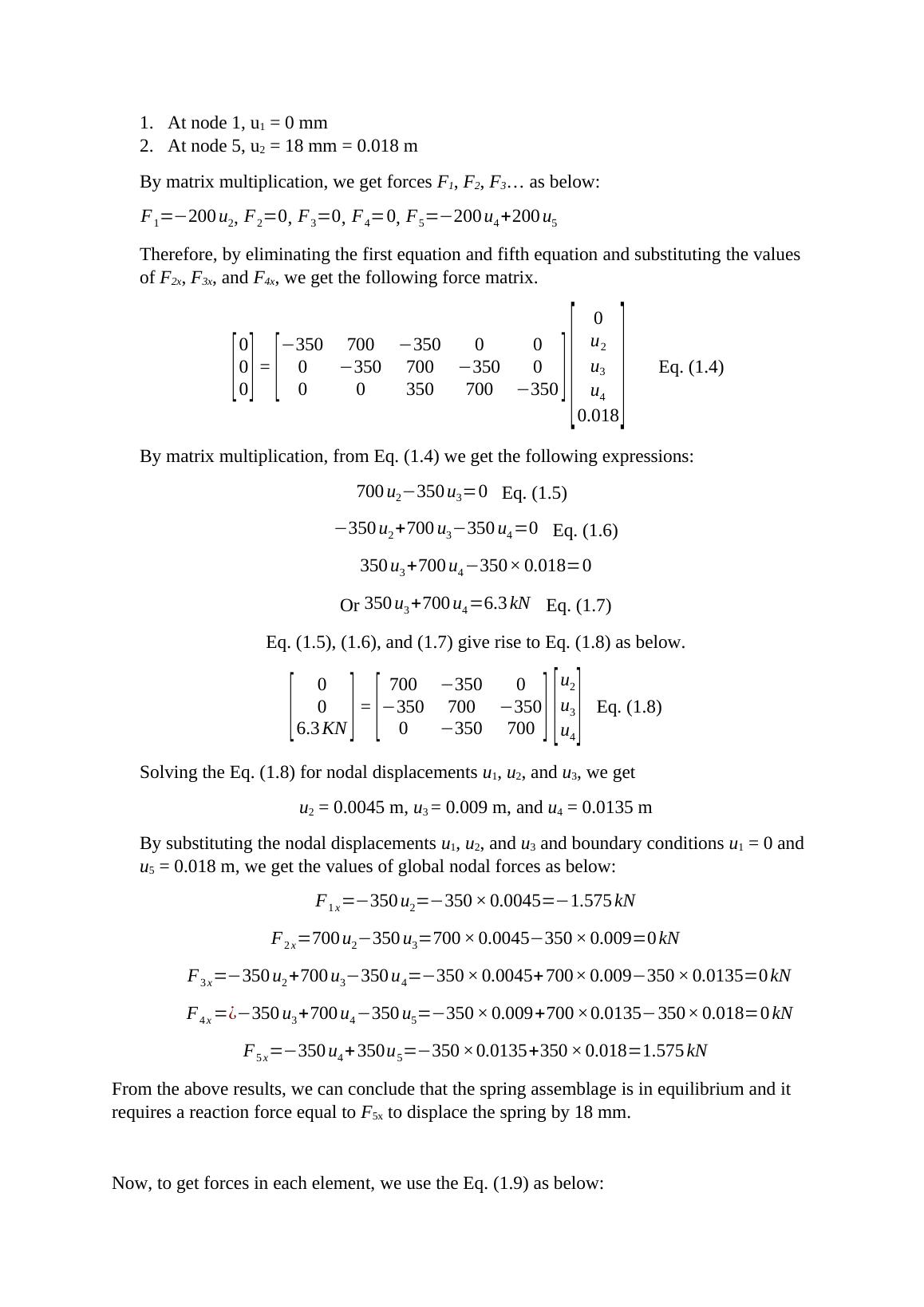
1.At node 1, u1 = 0 mm2.At node 5, u2 = 18 mm = 0.018 mBy matrix multiplication, we get forces F1, F2, F3... as below:F1=−200u2, F2=0, F3=0, F4=0, F5=−200u4+200u5Therefore, by eliminating the first equation and fifth equation and substituting the values of F2x, F3x, and F4x, we get the following force matrix.[000] = [−350700−350000−350700−350000350700−350][0u2u3u40.018]Eq. (1.4)By matrix multiplication, from Eq. (1.4) we get the following expressions:700u2−350u3=0Eq. (1.5)−350u2+700u3−350u4=0Eq. (1.6)350u3+700u4−350×0.018=0Or 350u3+700u4=6.3kNEq. (1.7)Eq. (1.5), (1.6), and (1.7) give rise to Eq. (1.8) as below.[006.3KN] = [700−3500−350700−3500−350700][u2u3u4]Eq. (1.8)Solving the Eq. (1.8) for nodal displacements u1, u2, and u3, we getu2 = 0.0045 m, u3 = 0.009 m, and u4 = 0.0135 mBy substituting the nodal displacements u1, u2, and u3 and boundary conditions u1 = 0 and u5 = 0.018 m, we get the values of global nodal forces as below:F1x=−350u2=−350×0.0045=−1.575kNF2x=700u2−350u3=700×0.0045−350×0.009=0kNF3x=−350u2+700u3−350u4=−350×0.0045+700×0.009−350×0.0135=0kNF4x=¿−350u3+700u4−350u5=−350×0.009+700×0.0135−350×0.018=0kNF5x=−350u4+350u5=−350×0.0135+350×0.018=1.575kNFrom the above results, we can conclude that the spring assemblage is in equilibrium and it requires a reaction force equal to F5x to displace the spring by 18 mm.Now, to get forces in each element, we use the Eq. (1.9) as below:
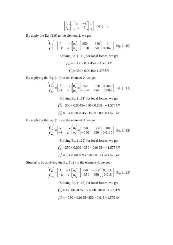
[f1xf2x]=[k−k−kk][u1u2] Eq. (1.9)By apply the Eq. (1.9) to the element 1, we get[f1x(1)f1x(2)]=[k−k−kk][u1u2]=[350−350−350350][00.0045] Eq. (1.10)Solving Eq. (1.10) for local forces, we getf1x(1)=−350×0.0045=−1.575kNf2x(1)=350×0.0045=1.575kNBy applying the Eq. (1.9) to the element 2, we get[f2x(2)f3x(2)]=[k−k−kk][u2u3]=[350−350−350350][0.00450.009] Eq. (1.11)Solving Eq. (1.11) for local forces, we getf2x(2)=350×0.0045−350×0.009=−1.575kNf3x(2)=−350×0.0045+350×0.009=1.575kNBy applying the Eq. (1.9) to the element 3, we get[f3x(3)f4x(3)]=[k−k−kk][u3u4]=[350−350−350350][0.0090.0135] Eq. (1.12)Solving Eq. (1.12) for local forces, we getf3x(3)=350×0.009−350×0.0135=−1.575kNf4x(3)=−350×0.009+350×0.0135=1.575kNSimilarly, by applying the Eq. (1.9) to the element 4, we get[f4x(4)f5x(4)]=[k−k−kk][u4u5]=[350−350−350350][0.01350.018] Eq. (1.13)Solving Eq. (1.13) for local forces, we getf4x(4)=350×0.0135−350×0.018=−1.575kNf5x(4)=−350×0.0135+350×0.018=1.575kN
End of preview
Want to access all the pages? Upload your documents or become a member.
Related Documents
Finite Element Analysis of a Truss Structurelg...
|9
|852
|184