Gram-Schmidt Process for QR Factorization of Matrix A in MATLAB | MATH 240
VerifiedAdded on 2023/05/29
|24
|3739
|277
AI Summary
This article explains how to perform Gram-Schmidt process for QR factorization of matrix A in MATLAB for MATH 240 course. It also covers how to compute rank of a matrix and form a basis for a subspace using MATLAB.
Contribute Materials
Your contribution can guide someone’s learning journey. Share your
documents today.
Running head: MATLAB PROJECT 4
MATH 240
MATLAB PROJECT 4
Name of the Student
Name of the University
Author Note
MATH 240
MATLAB PROJECT 4
Name of the Student
Name of the University
Author Note
Secure Best Marks with AI Grader
Need help grading? Try our AI Grader for instant feedback on your assignments.
1MATLAB PROJECT 4
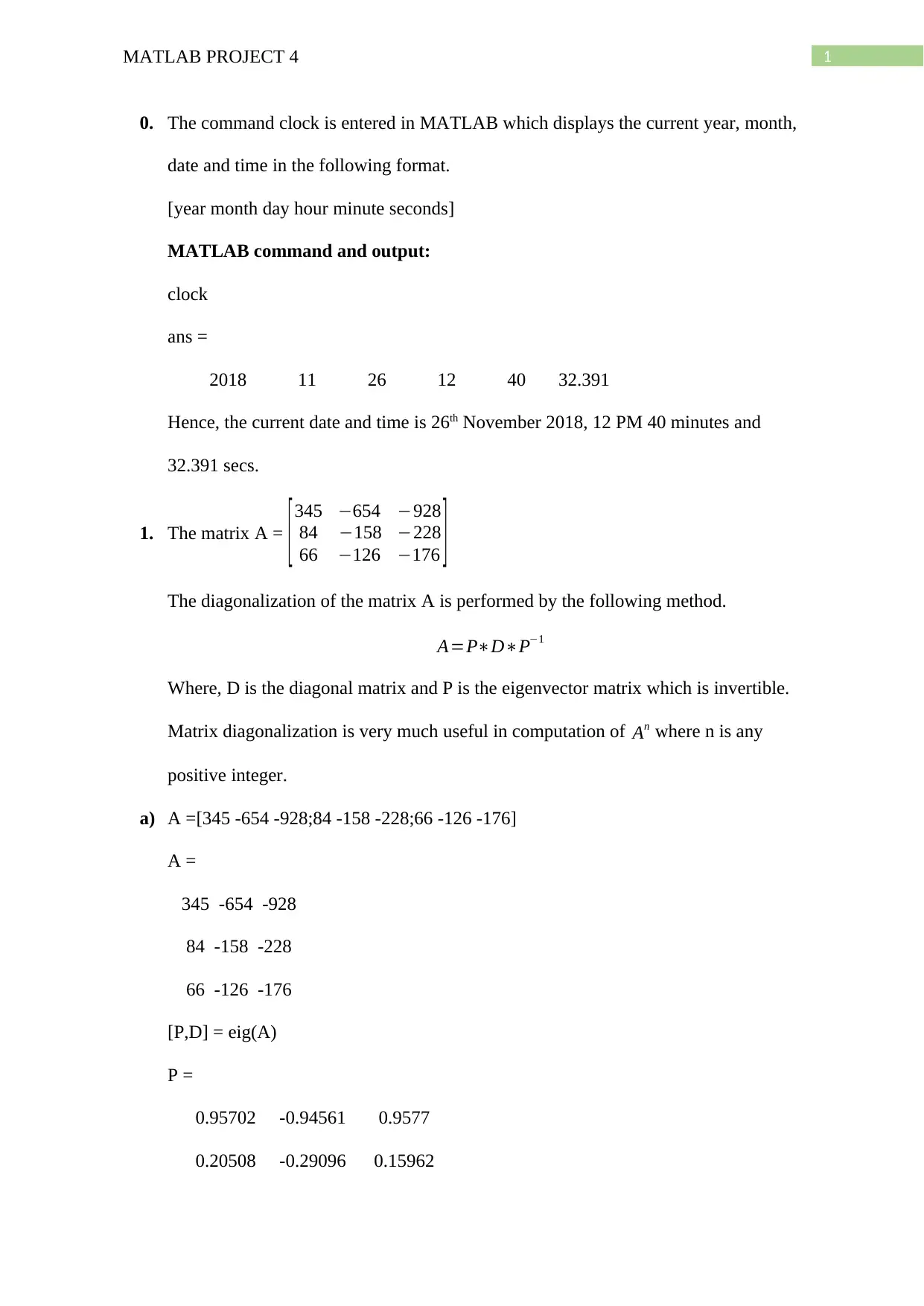
0. The command clock is entered in MATLAB which displays the current year, month,
date and time in the following format.
[year month day hour minute seconds]
MATLAB command and output:
clock
ans =
2018 11 26 12 40 32.391
Hence, the current date and time is 26th November 2018, 12 PM 40 minutes and
32.391 secs.
1. The matrix A = [ 345 −654 −928
84 −158 −228
66 −126 −176 ]
The diagonalization of the matrix A is performed by the following method.
A=P∗D∗P−1
Where, D is the diagonal matrix and P is the eigenvector matrix which is invertible.
Matrix diagonalization is very much useful in computation of An where n is any
positive integer.
a) A =[345 -654 -928;84 -158 -228;66 -126 -176]
A =
345 -654 -928
84 -158 -228
66 -126 -176
[P,D] = eig(A)
P =
0.95702 -0.94561 0.9577
0.20508 -0.29096 0.15962
2MATLAB PROJECT 4
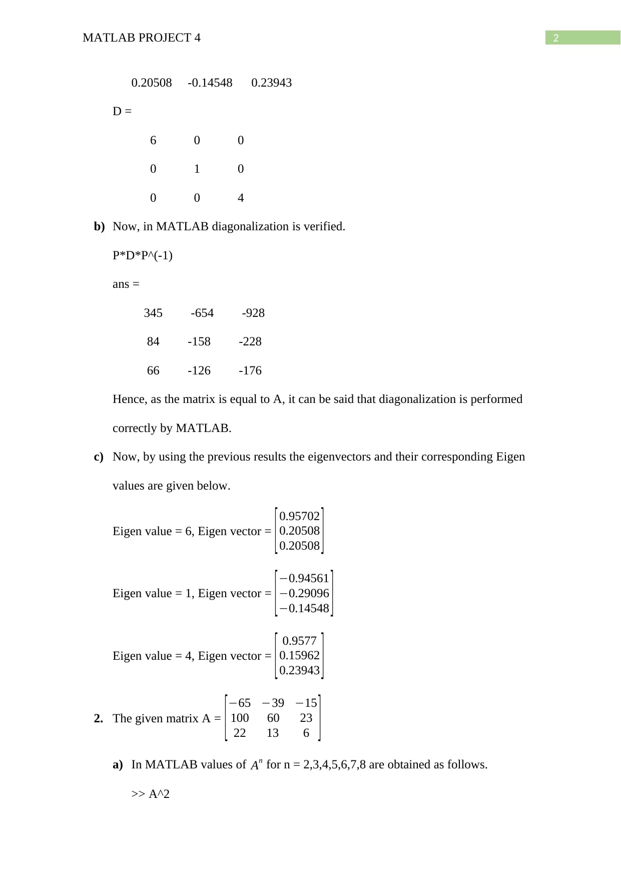
0.20508 -0.14548 0.23943
D =
6 0 0
0 1 0
0 0 4
b) Now, in MATLAB diagonalization is verified.
P*D*P^(-1)
ans =
345 -654 -928
84 -158 -228
66 -126 -176
Hence, as the matrix is equal to A, it can be said that diagonalization is performed
correctly by MATLAB.
c) Now, by using the previous results the eigenvectors and their corresponding Eigen
values are given below.
Eigen value = 6, Eigen vector = [0.95702
0.20508
0.20508 ]
Eigen value = 1, Eigen vector = [−0.94561
−0.29096
−0.14548 ]
Eigen value = 4, Eigen vector = [ 0.9577
0.15962
0.23943 ]
2. The given matrix A = [−65 −39 −15
100 60 23
22 13 6 ]
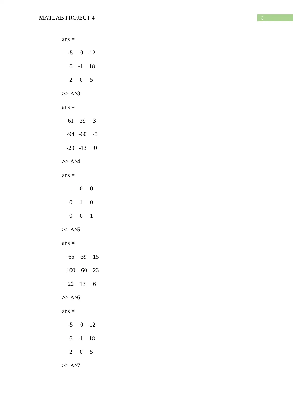
a) In MATLAB values of An for n = 2,3,4,5,6,7,8 are obtained as follows.
>> A^2
3MATLAB PROJECT 4
ans =
-5 0 -12
6 -1 18
2 0 5
>> A^3
ans =
61 39 3
-94 -60 -5
-20 -13 0
>> A^4
ans =
1 0 0
0 1 0
0 0 1
>> A^5
ans =
-65 -39 -15
100 60 23
22 13 6
>> A^6
ans =
-5 0 -12
6 -1 18
2 0 5
>> A^7
ans =
-5 0 -12
6 -1 18
2 0 5
>> A^3
ans =
61 39 3
-94 -60 -5
-20 -13 0
>> A^4
ans =
1 0 0
0 1 0
0 0 1
>> A^5
ans =
-65 -39 -15
100 60 23
22 13 6
>> A^6
ans =
-5 0 -12
6 -1 18
2 0 5
>> A^7
Secure Best Marks with AI Grader
Need help grading? Try our AI Grader for instant feedback on your assignments.
4MATLAB PROJECT 4
ans =
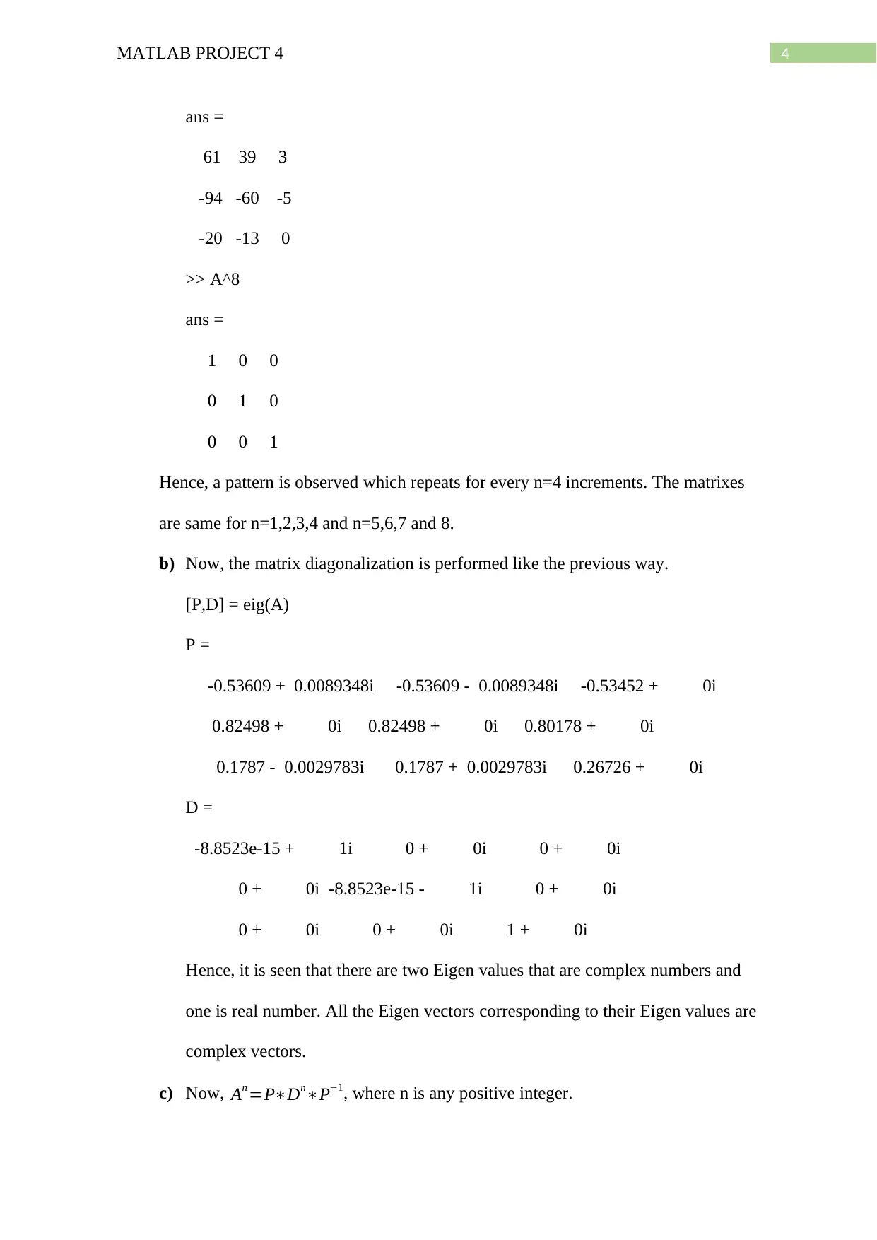
61 39 3
-94 -60 -5
-20 -13 0
>> A^8
ans =
1 0 0
0 1 0
0 0 1
Hence, a pattern is observed which repeats for every n=4 increments. The matrixes
are same for n=1,2,3,4 and n=5,6,7 and 8.
b) Now, the matrix diagonalization is performed like the previous way.
[P,D] = eig(A)
P =
-0.53609 + 0.0089348i -0.53609 - 0.0089348i -0.53452 + 0i
0.82498 + 0i 0.82498 + 0i 0.80178 + 0i
0.1787 - 0.0029783i 0.1787 + 0.0029783i 0.26726 + 0i
D =
-8.8523e-15 + 1i 0 + 0i 0 + 0i
0 + 0i -8.8523e-15 - 1i 0 + 0i
0 + 0i 0 + 0i 1 + 0i
Hence, it is seen that there are two Eigen values that are complex numbers and
one is real number. All the Eigen vectors corresponding to their Eigen values are
complex vectors.
c) Now, An =P∗Dn∗P−1, where n is any positive integer.
ans =
61 39 3
-94 -60 -5
-20 -13 0
>> A^8
ans =
1 0 0
0 1 0
0 0 1
Hence, a pattern is observed which repeats for every n=4 increments. The matrixes
are same for n=1,2,3,4 and n=5,6,7 and 8.
b) Now, the matrix diagonalization is performed like the previous way.
[P,D] = eig(A)
P =
-0.53609 + 0.0089348i -0.53609 - 0.0089348i -0.53452 + 0i
0.82498 + 0i 0.82498 + 0i 0.80178 + 0i
0.1787 - 0.0029783i 0.1787 + 0.0029783i 0.26726 + 0i
D =
-8.8523e-15 + 1i 0 + 0i 0 + 0i
0 + 0i -8.8523e-15 - 1i 0 + 0i
0 + 0i 0 + 0i 1 + 0i
Hence, it is seen that there are two Eigen values that are complex numbers and
one is real number. All the Eigen vectors corresponding to their Eigen values are
complex vectors.
c) Now, An =P∗Dn∗P−1, where n is any positive integer.
5MATLAB PROJECT 4
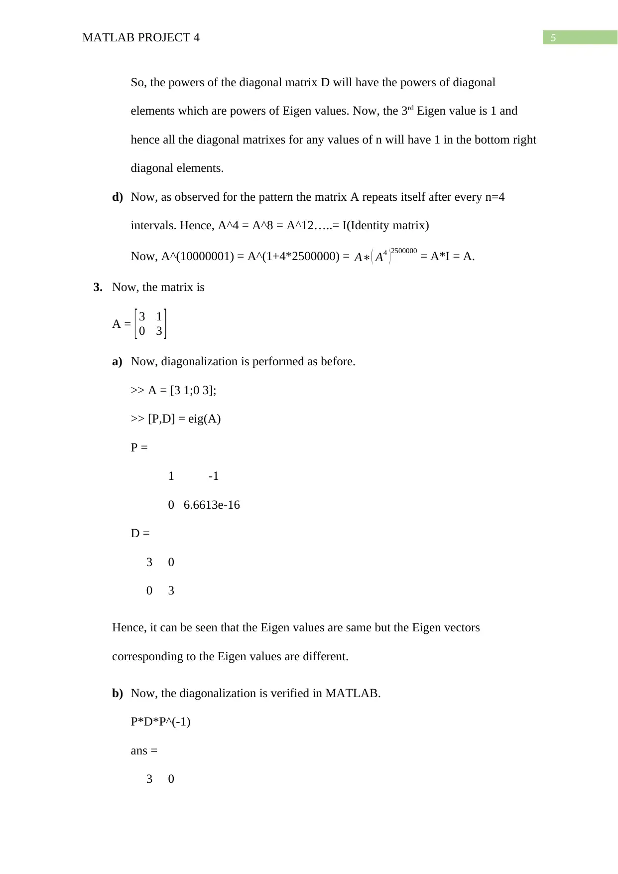
So, the powers of the diagonal matrix D will have the powers of diagonal
elements which are powers of Eigen values. Now, the 3rd Eigen value is 1 and
hence all the diagonal matrixes for any values of n will have 1 in the bottom right
diagonal elements.
d) Now, as observed for the pattern the matrix A repeats itself after every n=4
intervals. Hence, A^4 = A^8 = A^12…..= I(Identity matrix)
Now, A^(10000001) = A^(1+4*2500000) = A∗( A4 ) 2500000 = A*I = A.
3. Now, the matrix is
A = [ 3 1
0 3 ]
a) Now, diagonalization is performed as before.
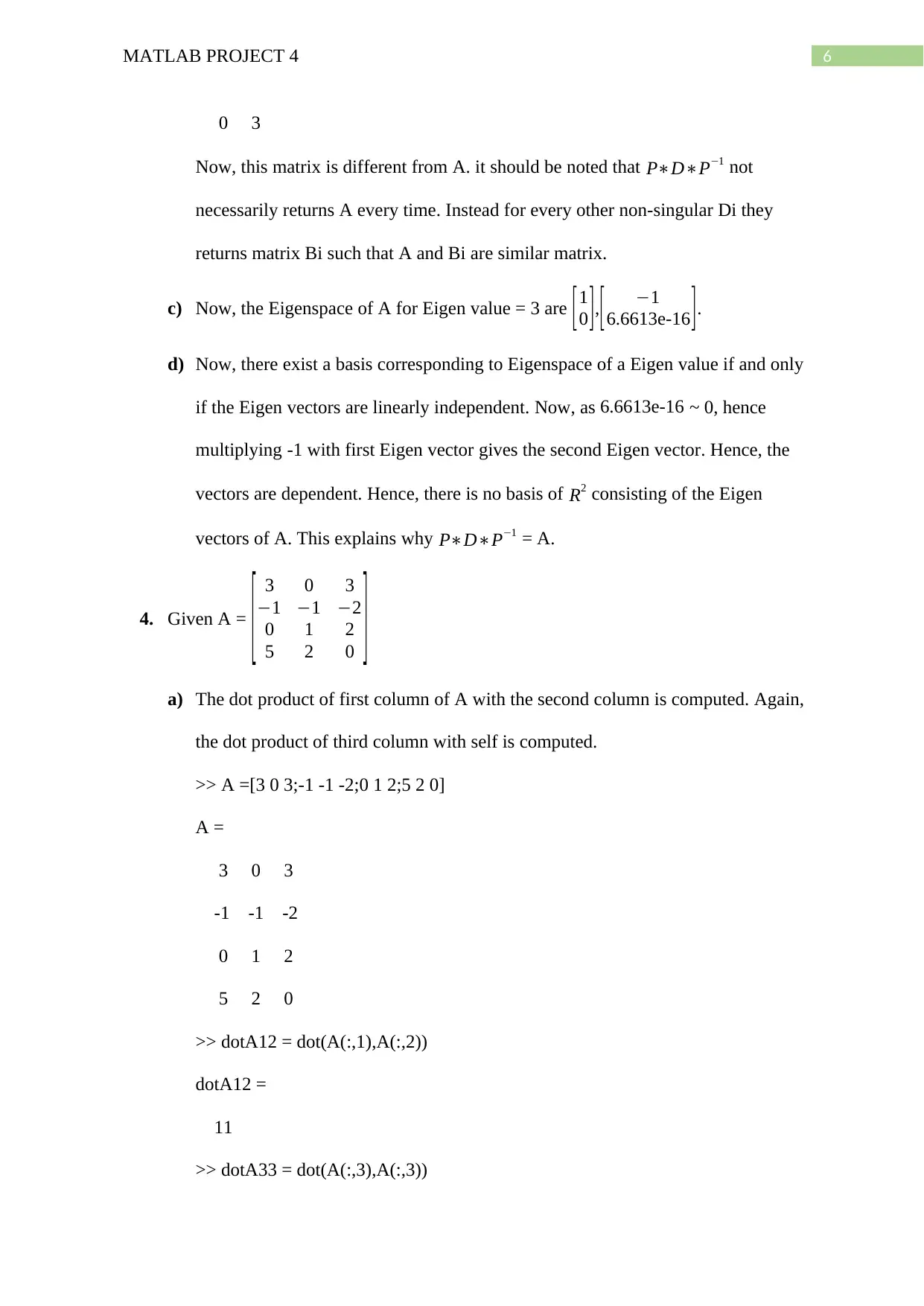
>> A = [3 1;0 3];
>> [P,D] = eig(A)
P =
1 -1
0 6.6613e-16
D =
3 0
0 3
Hence, it can be seen that the Eigen values are same but the Eigen vectors
corresponding to the Eigen values are different.
b) Now, the diagonalization is verified in MATLAB.
P*D*P^(-1)
ans =
3 0
6MATLAB PROJECT 4
0 3
Now, this matrix is different from A. it should be noted that P∗D∗P−1 not
necessarily returns A every time. Instead for every other non-singular Di they
returns matrix Bi such that A and Bi are similar matrix.
c) Now, the Eigenspace of A for Eigen value = 3 are [ 1
0 ],[ −1
6.6613e-16 ].
d) Now, there exist a basis corresponding to Eigenspace of a Eigen value if and only
if the Eigen vectors are linearly independent. Now, as 6.6613e-16 ~ 0, hence
multiplying -1 with first Eigen vector gives the second Eigen vector. Hence, the
vectors are dependent. Hence, there is no basis of R2 consisting of the Eigen
vectors of A. This explains why P∗D∗P−1 = A.
4. Given A =
[ 3 0 3
−1 −1 −2
0 1 2
5 2 0 ]
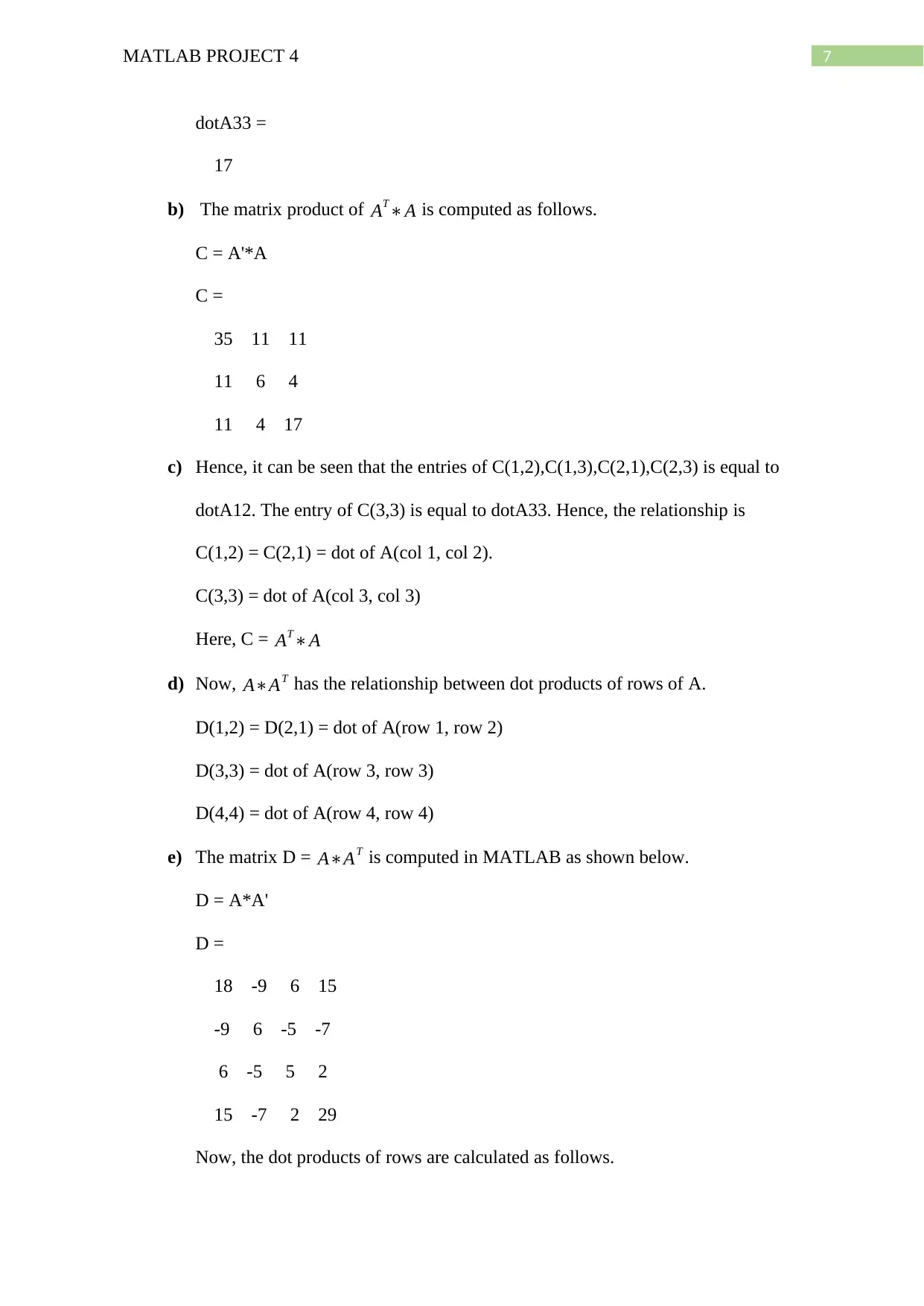
a) The dot product of first column of A with the second column is computed. Again,
the dot product of third column with self is computed.
>> A =[3 0 3;-1 -1 -2;0 1 2;5 2 0]
A =
3 0 3
-1 -1 -2
0 1 2
5 2 0
>> dotA12 = dot(A(:,1),A(:,2))
dotA12 =
11
>> dotA33 = dot(A(:,3),A(:,3))
Paraphrase This Document
Need a fresh take? Get an instant paraphrase of this document with our AI Paraphraser
7MATLAB PROJECT 4
dotA33 =
17
b) The matrix product of AT∗A is computed as follows.
C = A'*A
C =
35 11 11
11 6 4
11 4 17
c) Hence, it can be seen that the entries of C(1,2),C(1,3),C(2,1),C(2,3) is equal to
dotA12. The entry of C(3,3) is equal to dotA33. Hence, the relationship is
C(1,2) = C(2,1) = dot of A(col 1, col 2).
C(3,3) = dot of A(col 3, col 3)
Here, C = AT∗A
d) Now, A∗AT has the relationship between dot products of rows of A.
D(1,2) = D(2,1) = dot of A(row 1, row 2)
D(3,3) = dot of A(row 3, row 3)
D(4,4) = dot of A(row 4, row 4)
e) The matrix D = A∗AT is computed in MATLAB as shown below.
D = A*A'
D =
18 -9 6 15
-9 6 -5 -7
6 -5 5 2
15 -7 2 29
Now, the dot products of rows are calculated as follows.
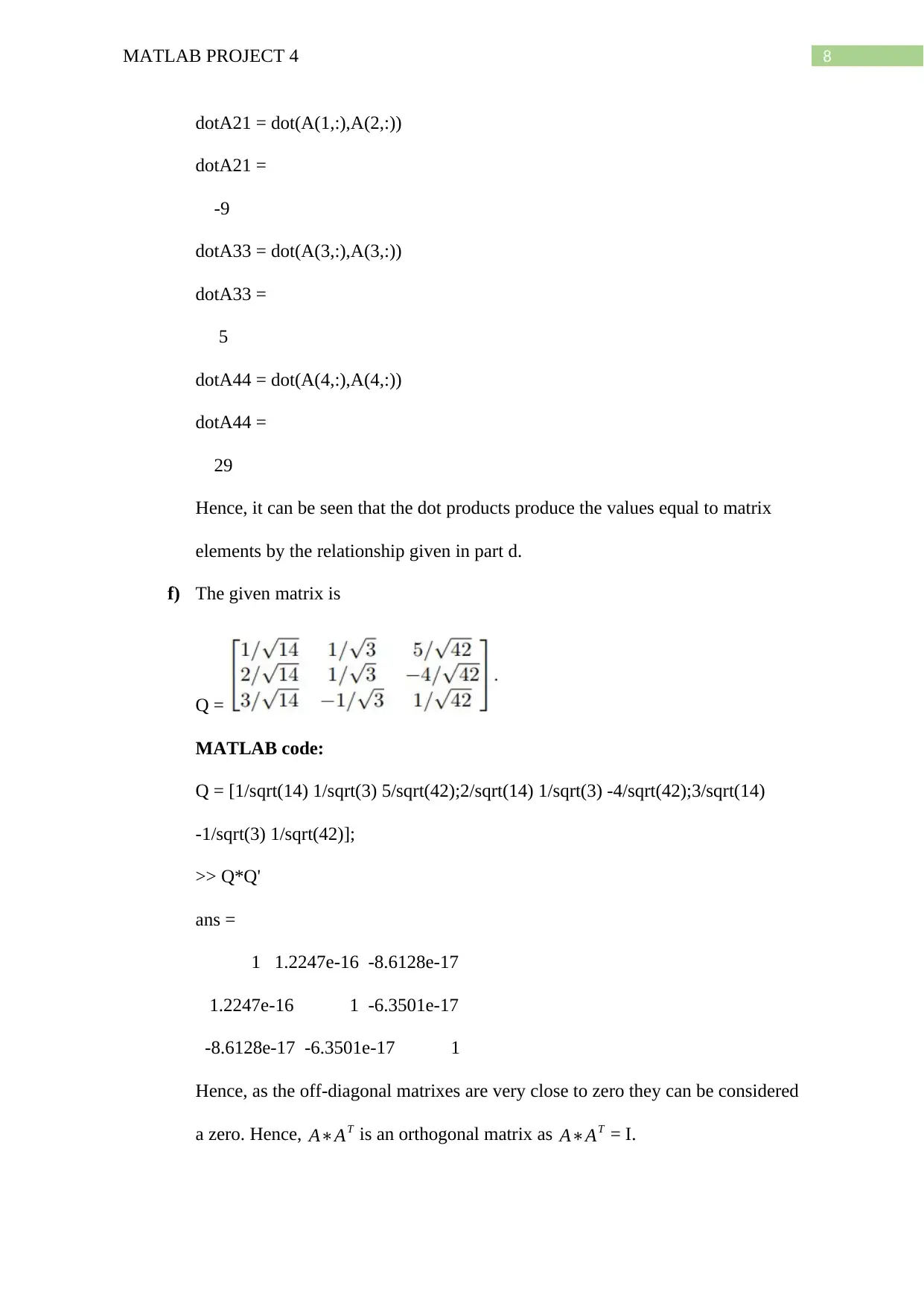
8MATLAB PROJECT 4
dotA21 = dot(A(1,:),A(2,:))
dotA21 =
-9
dotA33 = dot(A(3,:),A(3,:))
dotA33 =
5
dotA44 = dot(A(4,:),A(4,:))
dotA44 =
29
Hence, it can be seen that the dot products produce the values equal to matrix
elements by the relationship given in part d.
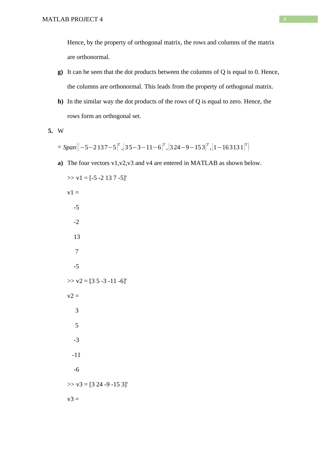
f) The given matrix is
Q =
MATLAB code:
Q = [1/sqrt(14) 1/sqrt(3) 5/sqrt(42);2/sqrt(14) 1/sqrt(3) -4/sqrt(42);3/sqrt(14)
-1/sqrt(3) 1/sqrt(42)];
>> Q*Q'
ans =
1 1.2247e-16 -8.6128e-17
1.2247e-16 1 -6.3501e-17
-8.6128e-17 -6.3501e-17 1
Hence, as the off-diagonal matrixes are very close to zero they can be considered
a zero. Hence, A∗AT is an orthogonal matrix as A∗AT = I.
9MATLAB PROJECT 4
Hence, by the property of orthogonal matrix, the rows and columns of the matrix
are orthonormal.
g) It can be seen that the dot products between the columns of Q is equal to 0. Hence,
the columns are orthonormal. This leads from the property of orthogonal matrix.
h) In the similar way the dot products of the rows of Q is equal to zero. Hence, the
rows form an orthogonal set.
5. W
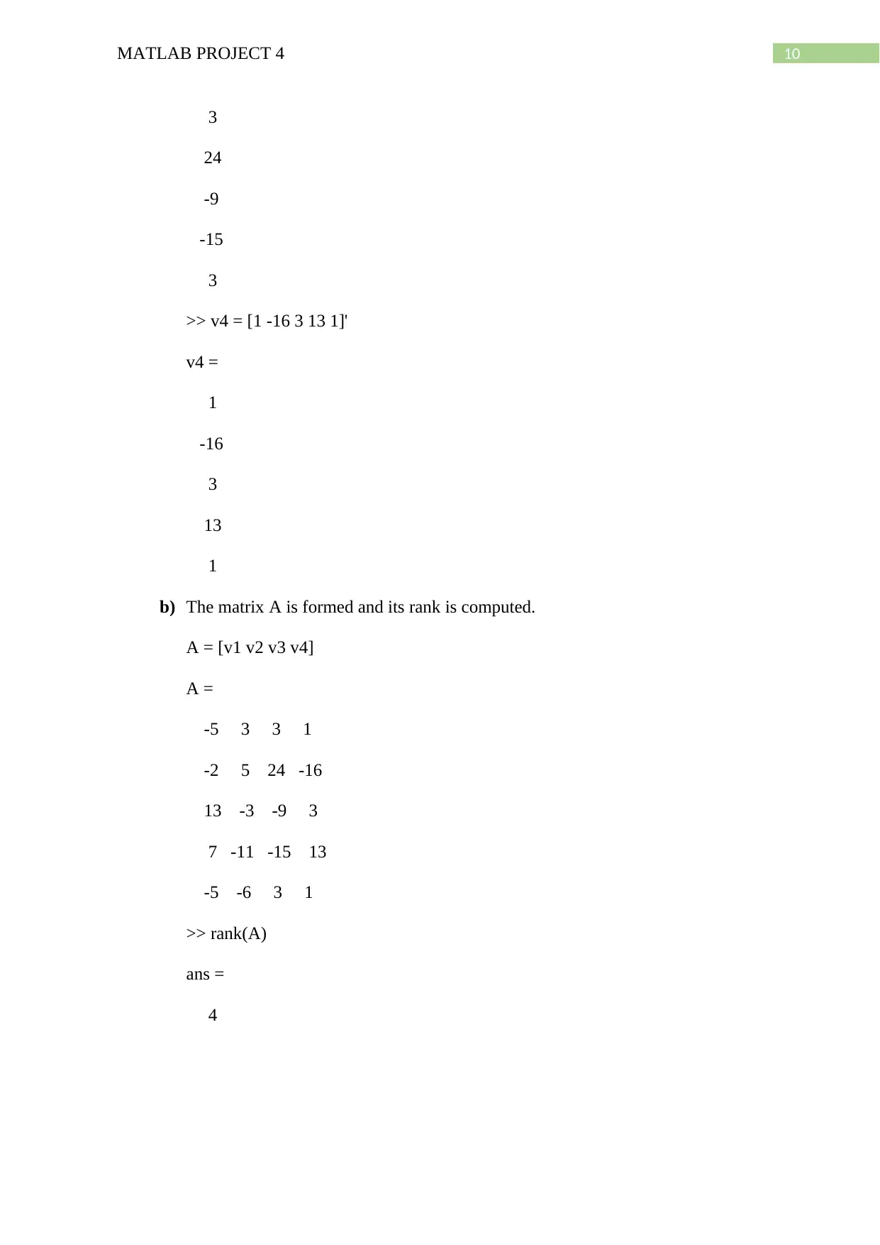
= Span ( [−5−2 13 7−5 ]T , [ 3 5−3−11−6 ]T , [3 24−9−15 3 ] T , [1−16 313 1 ] T )
a) The four vectors v1,v2,v3 and v4 are entered in MATLAB as shown below.
>> v1 = [-5 -2 13 7 -5]'
v1 =
-5
-2
13
7
-5
>> v2 = [3 5 -3 -11 -6]'
v2 =
3
5
-3
-11
-6
>> v3 = [3 24 -9 -15 3]'
v3 =
Secure Best Marks with AI Grader
Need help grading? Try our AI Grader for instant feedback on your assignments.
10MATLAB PROJECT 4
3
24
-9
-15
3
>> v4 = [1 -16 3 13 1]'
v4 =
1
-16
3
13
1
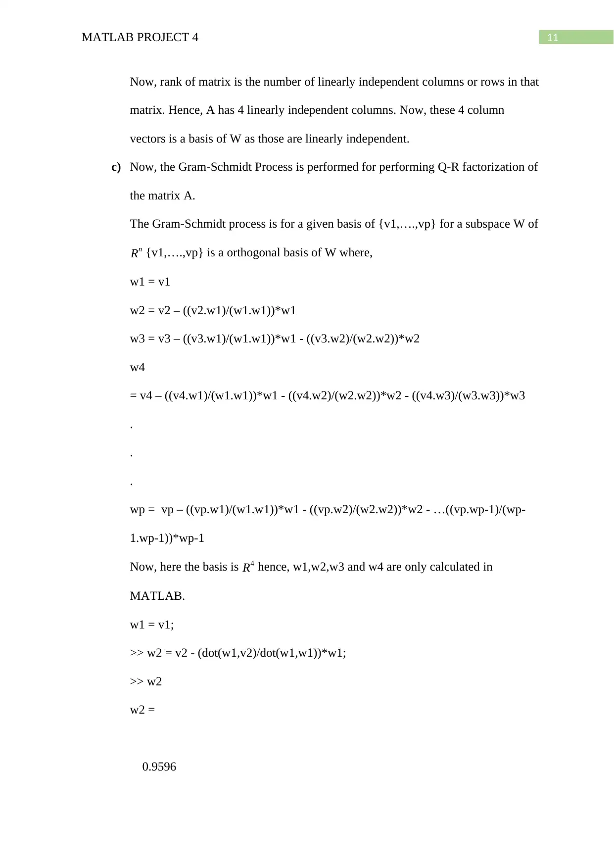
b) The matrix A is formed and its rank is computed.
A = [v1 v2 v3 v4]
A =
-5 3 3 1
-2 5 24 -16
13 -3 -9 3
7 -11 -15 13
-5 -6 3 1
>> rank(A)
ans =
4
3
24
-9
-15
3
>> v4 = [1 -16 3 13 1]'
v4 =
1
-16
3
13
1
b) The matrix A is formed and its rank is computed.
A = [v1 v2 v3 v4]
A =
-5 3 3 1
-2 5 24 -16
13 -3 -9 3
7 -11 -15 13
-5 -6 3 1
>> rank(A)
ans =
4
11MATLAB PROJECT 4
Now, rank of matrix is the number of linearly independent columns or rows in that
matrix. Hence, A has 4 linearly independent columns. Now, these 4 column
vectors is a basis of W as those are linearly independent.
c) Now, the Gram-Schmidt Process is performed for performing Q-R factorization of
the matrix A.
The Gram-Schmidt process is for a given basis of {v1,….,vp} for a subspace W of
Rn {v1,….,vp} is a orthogonal basis of W where,
w1 = v1
w2 = v2 – ((v2.w1)/(w1.w1))*w1
w3 = v3 – ((v3.w1)/(w1.w1))*w1 - ((v3.w2)/(w2.w2))*w2
w4
= v4 – ((v4.w1)/(w1.w1))*w1 - ((v4.w2)/(w2.w2))*w2 - ((v4.w3)/(w3.w3))*w3
.
.
.
wp = vp – ((vp.w1)/(w1.w1))*w1 - ((vp.w2)/(w2.w2))*w2 - …((vp.wp-1)/(wp-
1.wp-1))*wp-1
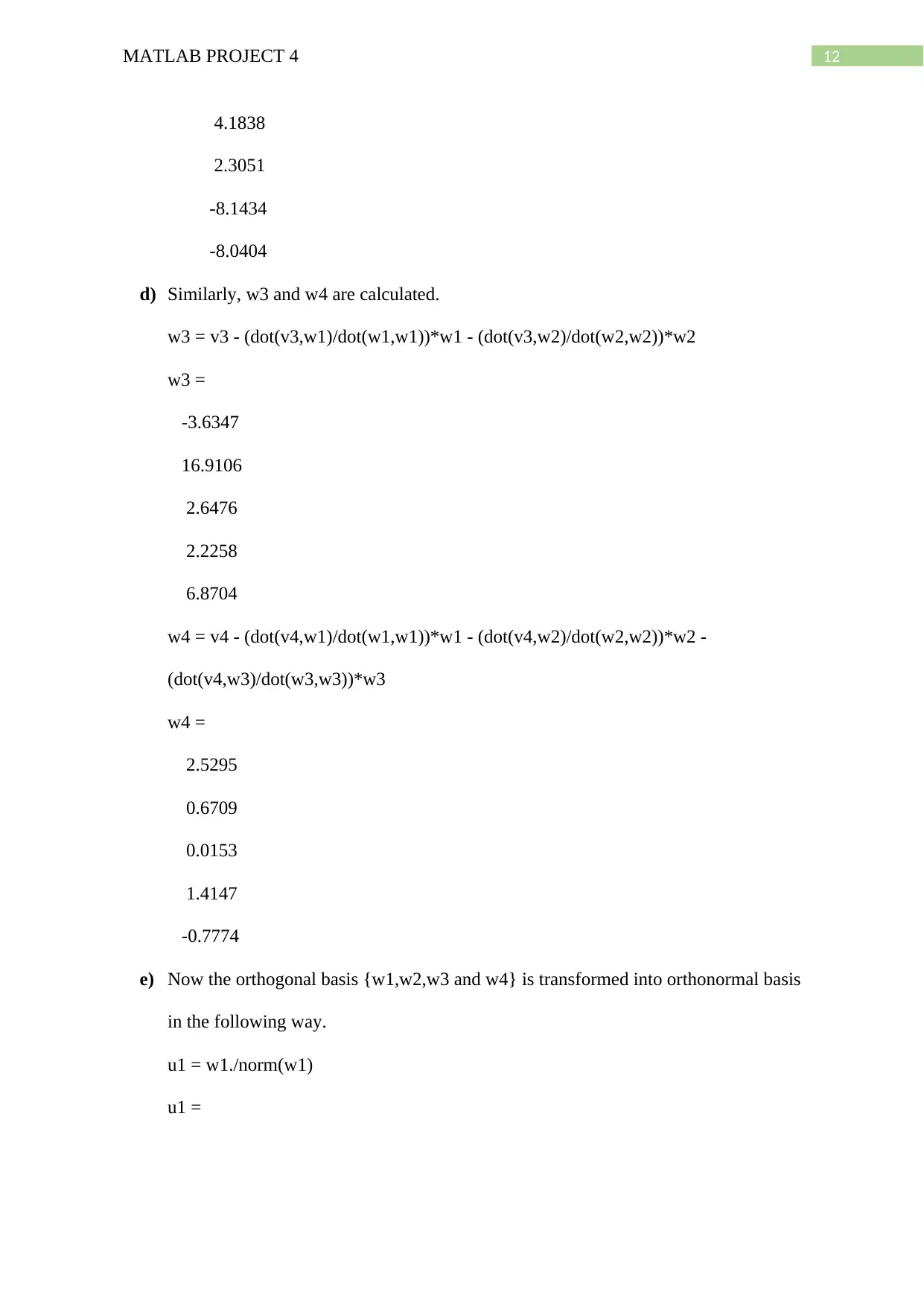
Now, here the basis is R4 hence, w1,w2,w3 and w4 are only calculated in
MATLAB.
w1 = v1;
>> w2 = v2 - (dot(w1,v2)/dot(w1,w1))*w1;
>> w2
w2 =
0.9596
12MATLAB PROJECT 4
4.1838
2.3051
-8.1434
-8.0404
d) Similarly, w3 and w4 are calculated.
w3 = v3 - (dot(v3,w1)/dot(w1,w1))*w1 - (dot(v3,w2)/dot(w2,w2))*w2
w3 =
-3.6347
16.9106
2.6476
2.2258
6.8704
w4 = v4 - (dot(v4,w1)/dot(w1,w1))*w1 - (dot(v4,w2)/dot(w2,w2))*w2 -
(dot(v4,w3)/dot(w3,w3))*w3
w4 =
2.5295
0.6709
0.0153
1.4147
-0.7774
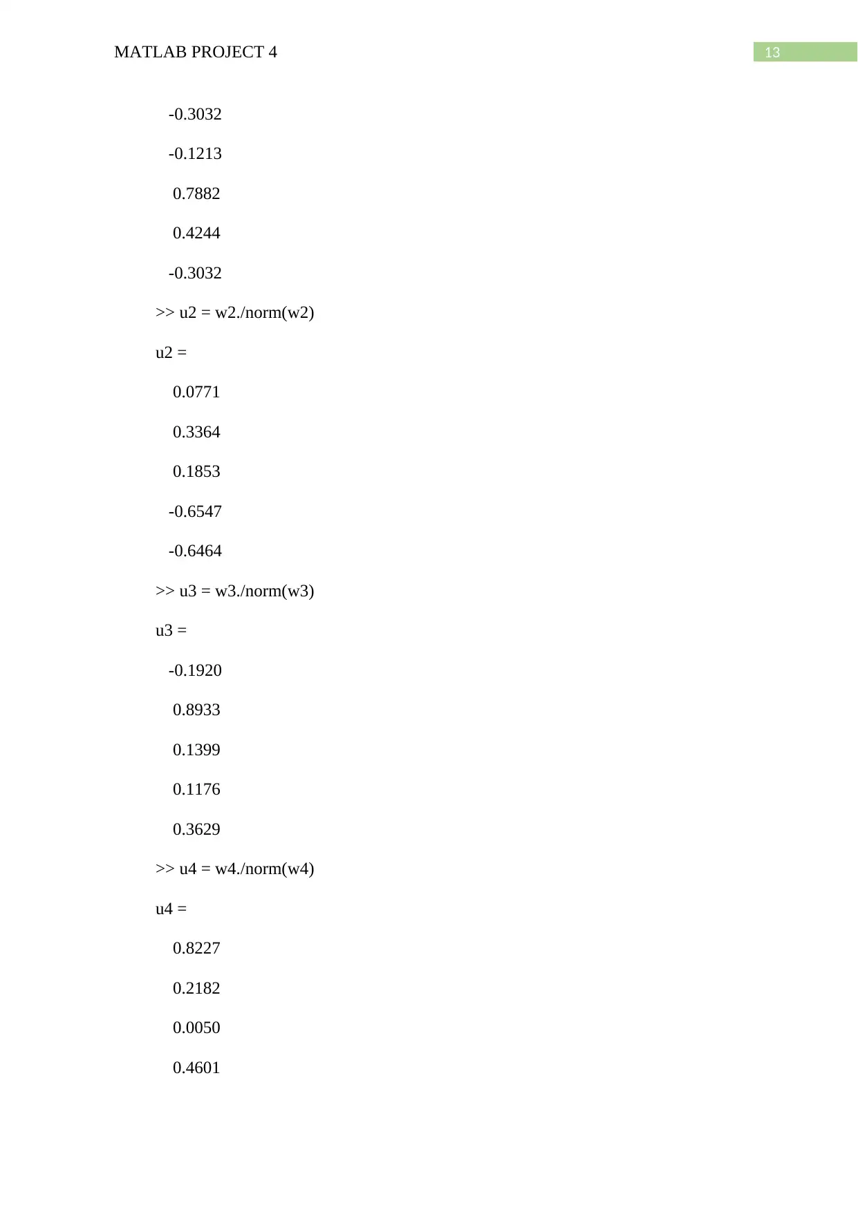
e) Now the orthogonal basis {w1,w2,w3 and w4} is transformed into orthonormal basis
in the following way.
u1 = w1./norm(w1)
u1 =
Paraphrase This Document
Need a fresh take? Get an instant paraphrase of this document with our AI Paraphraser
13MATLAB PROJECT 4
-0.3032
-0.1213
0.7882
0.4244
-0.3032
>> u2 = w2./norm(w2)
u2 =
0.0771
0.3364
0.1853
-0.6547
-0.6464
>> u3 = w3./norm(w3)
u3 =
-0.1920
0.8933
0.1399
0.1176
0.3629
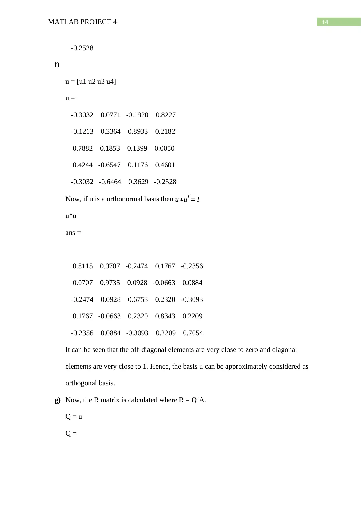
>> u4 = w4./norm(w4)
u4 =
0.8227
0.2182
0.0050
0.4601
-0.3032
-0.1213
0.7882
0.4244
-0.3032
>> u2 = w2./norm(w2)
u2 =
0.0771
0.3364
0.1853
-0.6547
-0.6464
>> u3 = w3./norm(w3)
u3 =
-0.1920
0.8933
0.1399
0.1176
0.3629
>> u4 = w4./norm(w4)
u4 =
0.8227
0.2182
0.0050
0.4601
14MATLAB PROJECT 4
-0.2528
f)
u = [u1 u2 u3 u4]
u =
-0.3032 0.0771 -0.1920 0.8227
-0.1213 0.3364 0.8933 0.2182
0.7882 0.1853 0.1399 0.0050
0.4244 -0.6547 0.1176 0.4601
-0.3032 -0.6464 0.3629 -0.2528
Now, if u is a orthonormal basis then u∗uT =I
u*u'
ans =
0.8115 0.0707 -0.2474 0.1767 -0.2356
0.0707 0.9735 0.0928 -0.0663 0.0884
-0.2474 0.0928 0.6753 0.2320 -0.3093
0.1767 -0.0663 0.2320 0.8343 0.2209
-0.2356 0.0884 -0.3093 0.2209 0.7054
It can be seen that the off-diagonal elements are very close to zero and diagonal
elements are very close to 1. Hence, the basis u can be approximately considered as
orthogonal basis.
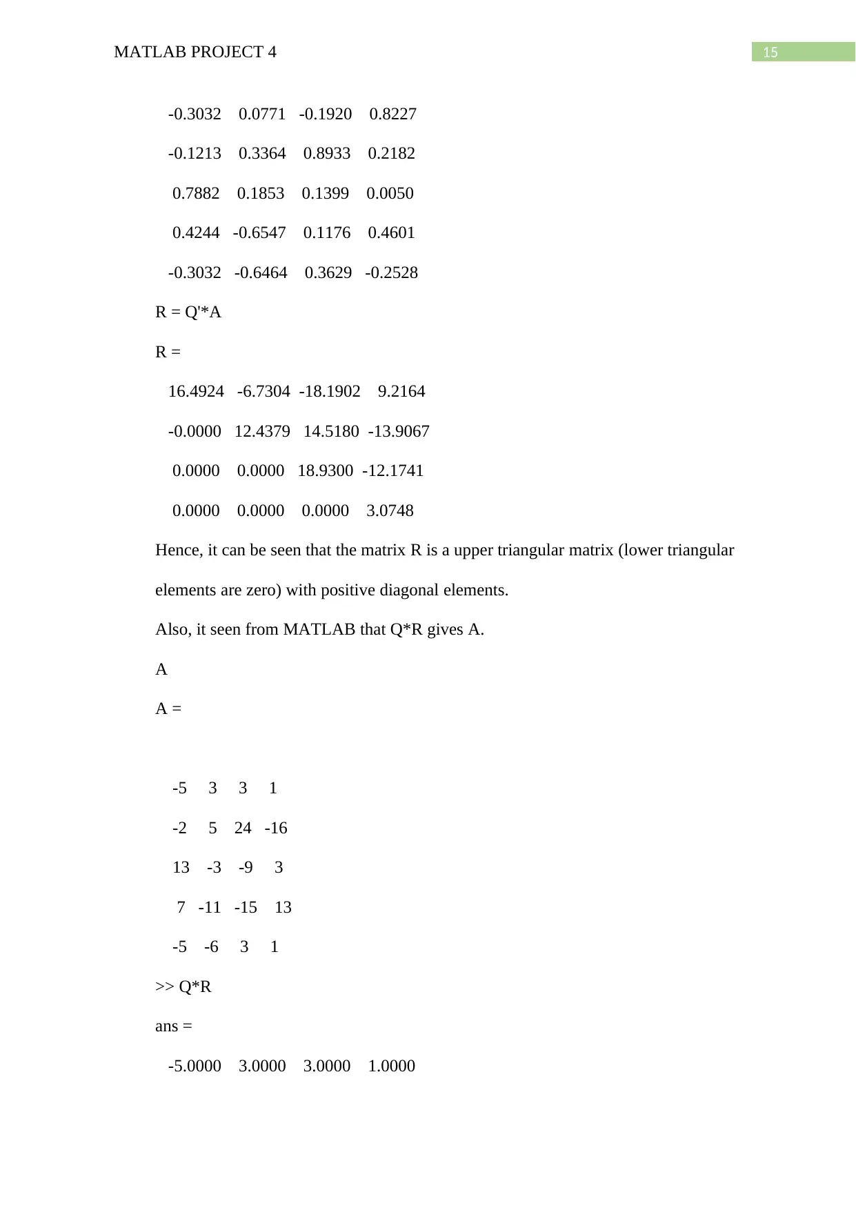
g) Now, the R matrix is calculated where R = Q’A.
Q = u
Q =
15MATLAB PROJECT 4
-0.3032 0.0771 -0.1920 0.8227
-0.1213 0.3364 0.8933 0.2182
0.7882 0.1853 0.1399 0.0050
0.4244 -0.6547 0.1176 0.4601
-0.3032 -0.6464 0.3629 -0.2528
R = Q'*A
R =
16.4924 -6.7304 -18.1902 9.2164
-0.0000 12.4379 14.5180 -13.9067
0.0000 0.0000 18.9300 -12.1741
0.0000 0.0000 0.0000 3.0748
Hence, it can be seen that the matrix R is a upper triangular matrix (lower triangular
elements are zero) with positive diagonal elements.
Also, it seen from MATLAB that Q*R gives A.
A
A =
-5 3 3 1
-2 5 24 -16
13 -3 -9 3
7 -11 -15 13
-5 -6 3 1
>> Q*R
ans =
-5.0000 3.0000 3.0000 1.0000
Secure Best Marks with AI Grader
Need help grading? Try our AI Grader for instant feedback on your assignments.
16MATLAB PROJECT 4
-2.0000 5.0000 24.0000 -16.0000
13.0000 -3.0000 -9.0000 3.0000
7.0000 -11.0000 -15.0000 13.0000
-5.0000 -6.0000 3.0000 1.0000
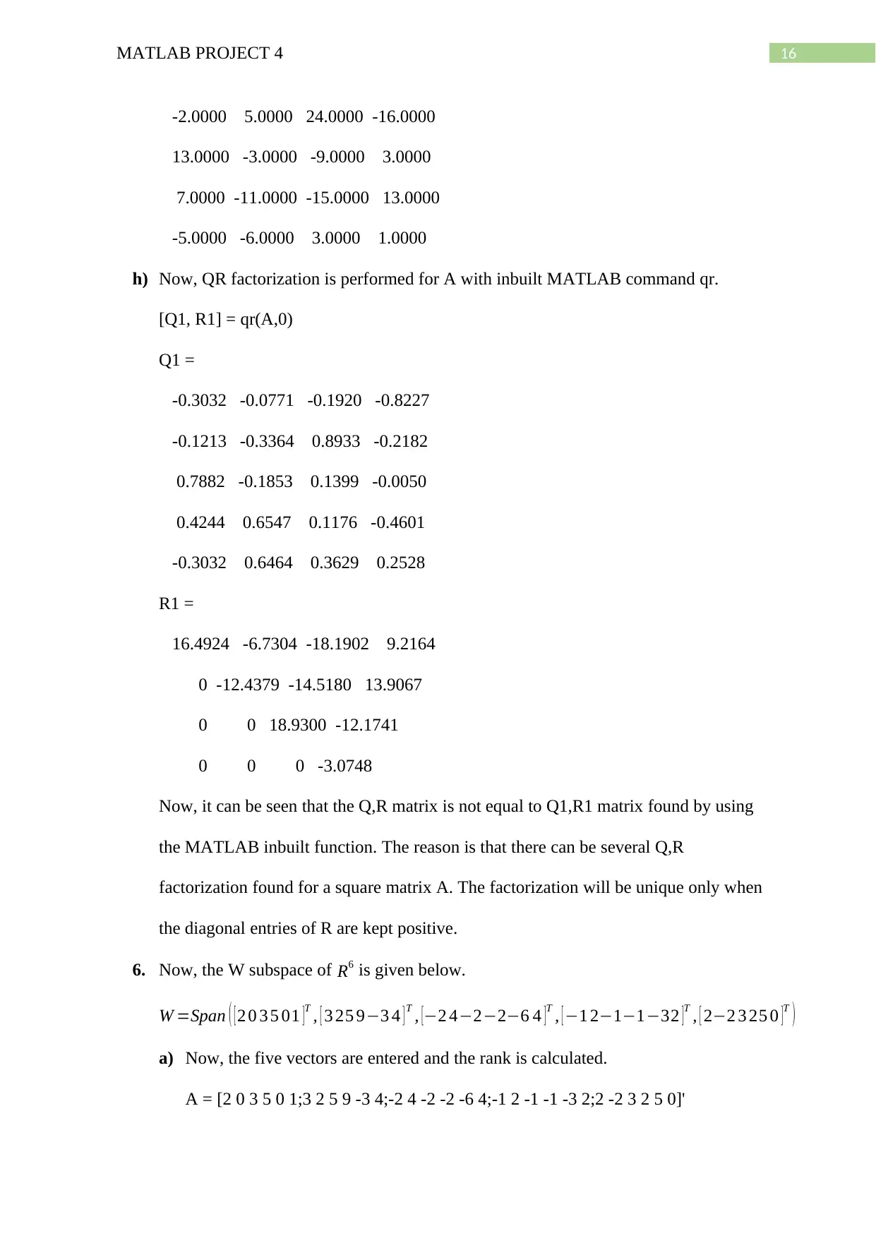
h) Now, QR factorization is performed for A with inbuilt MATLAB command qr.
[Q1, R1] = qr(A,0)
Q1 =
-0.3032 -0.0771 -0.1920 -0.8227
-0.1213 -0.3364 0.8933 -0.2182
0.7882 -0.1853 0.1399 -0.0050
0.4244 0.6547 0.1176 -0.4601
-0.3032 0.6464 0.3629 0.2528
R1 =
16.4924 -6.7304 -18.1902 9.2164
0 -12.4379 -14.5180 13.9067
0 0 18.9300 -12.1741
0 0 0 -3.0748
Now, it can be seen that the Q,R matrix is not equal to Q1,R1 matrix found by using
the MATLAB inbuilt function. The reason is that there can be several Q,R
factorization found for a square matrix A. The factorization will be unique only when
the diagonal entries of R are kept positive.
6. Now, the W subspace of R6 is given below.
W =Span ( [ 2 0 3 5 01 ]
T , [ 3 25 9−3 4 ] T , [−2 4−2−2−6 4 ]
T , [ −1 2−1−1−32 ]
T , [ 2−2 3 25 0 ]
T )
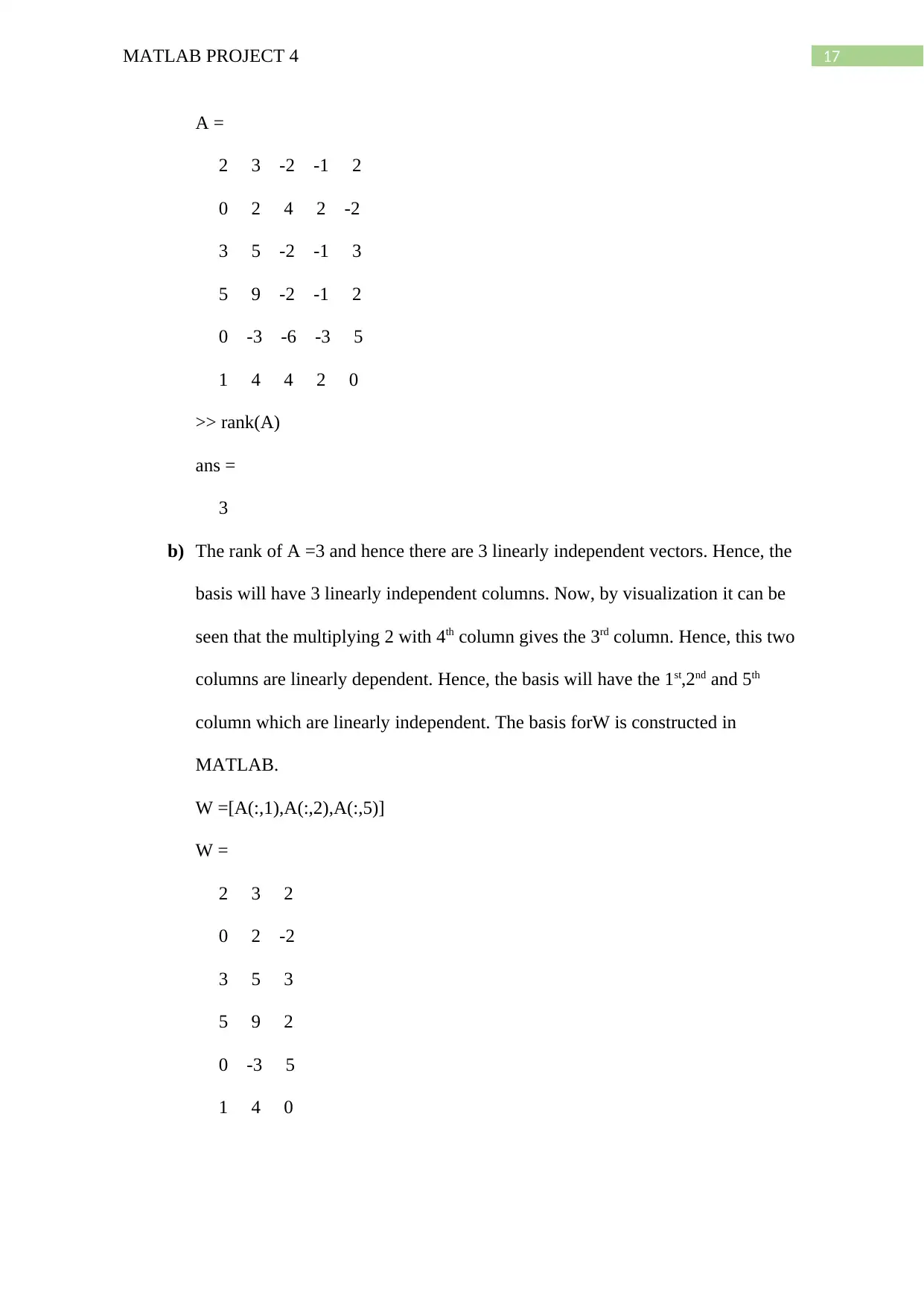
a) Now, the five vectors are entered and the rank is calculated.
A = [2 0 3 5 0 1;3 2 5 9 -3 4;-2 4 -2 -2 -6 4;-1 2 -1 -1 -3 2;2 -2 3 2 5 0]'
17MATLAB PROJECT 4
A =
2 3 -2 -1 2
0 2 4 2 -2
3 5 -2 -1 3
5 9 -2 -1 2
0 -3 -6 -3 5
1 4 4 2 0
>> rank(A)
ans =
3
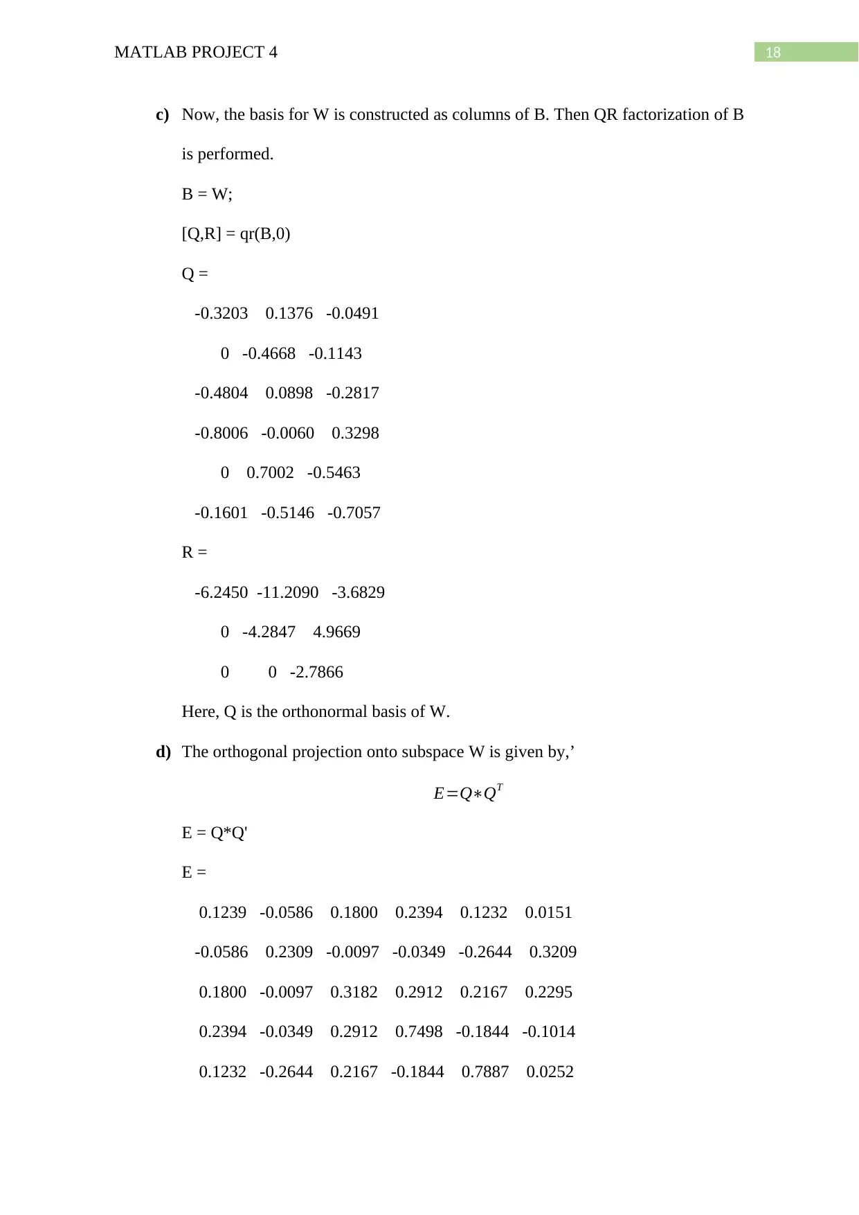
b) The rank of A =3 and hence there are 3 linearly independent vectors. Hence, the
basis will have 3 linearly independent columns. Now, by visualization it can be
seen that the multiplying 2 with 4th column gives the 3rd column. Hence, this two
columns are linearly dependent. Hence, the basis will have the 1st,2nd and 5th
column which are linearly independent. The basis forW is constructed in
MATLAB.
W =[A(:,1),A(:,2),A(:,5)]
W =
2 3 2
0 2 -2
3 5 3
5 9 2
0 -3 5
1 4 0
18MATLAB PROJECT 4
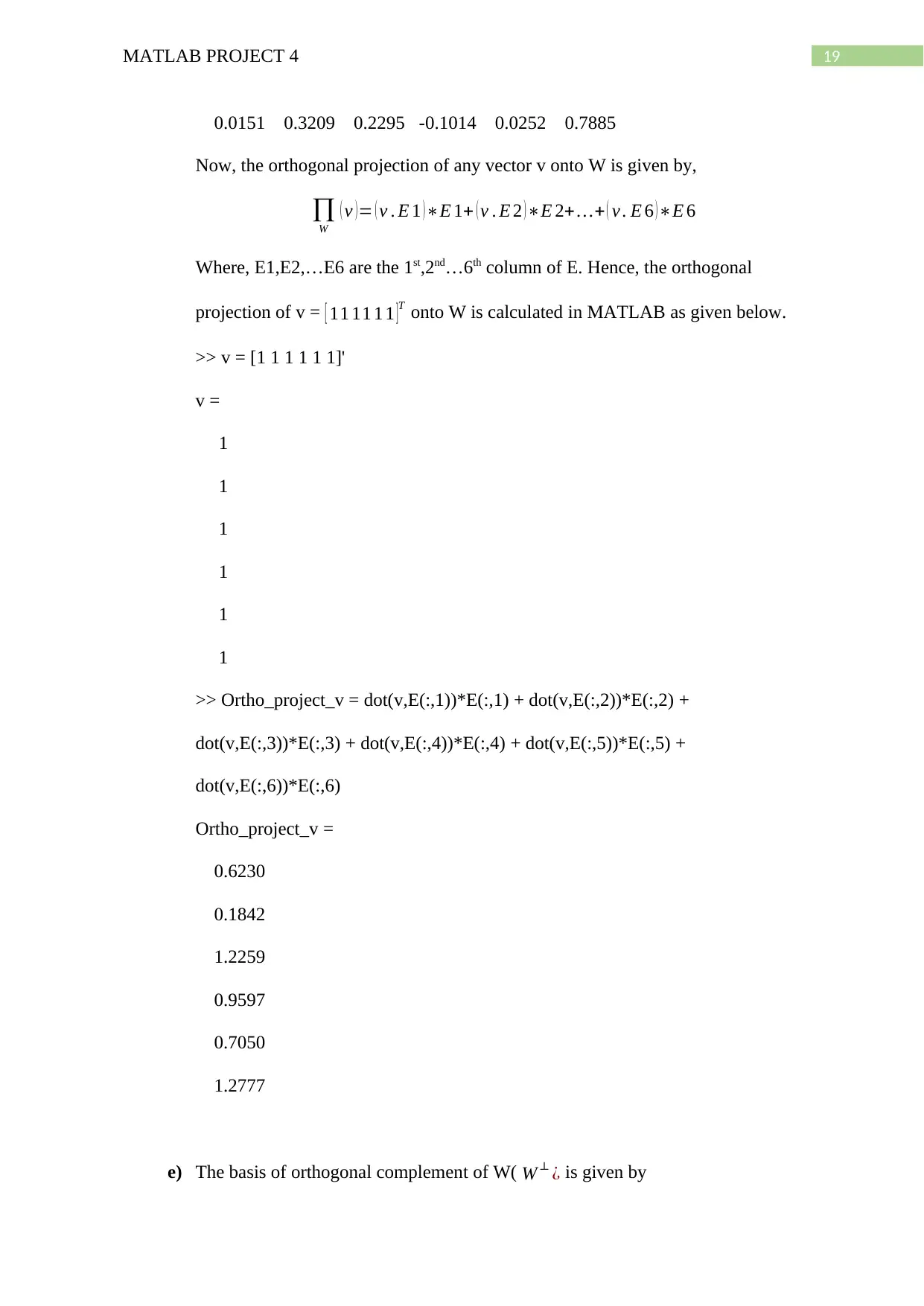
c) Now, the basis for W is constructed as columns of B. Then QR factorization of B
is performed.
B = W;
[Q,R] = qr(B,0)
Q =
-0.3203 0.1376 -0.0491
0 -0.4668 -0.1143
-0.4804 0.0898 -0.2817
-0.8006 -0.0060 0.3298
0 0.7002 -0.5463
-0.1601 -0.5146 -0.7057
R =
-6.2450 -11.2090 -3.6829
0 -4.2847 4.9669
0 0 -2.7866
Here, Q is the orthonormal basis of W.
d) The orthogonal projection onto subspace W is given by,’
E=Q∗QT
E = Q*Q'
E =
0.1239 -0.0586 0.1800 0.2394 0.1232 0.0151
-0.0586 0.2309 -0.0097 -0.0349 -0.2644 0.3209
0.1800 -0.0097 0.3182 0.2912 0.2167 0.2295
0.2394 -0.0349 0.2912 0.7498 -0.1844 -0.1014
0.1232 -0.2644 0.2167 -0.1844 0.7887 0.0252
Paraphrase This Document
Need a fresh take? Get an instant paraphrase of this document with our AI Paraphraser
19MATLAB PROJECT 4
0.0151 0.3209 0.2295 -0.1014 0.0252 0.7885
Now, the orthogonal projection of any vector v onto W is given by,
∏W
( v ) = ( v . E 1 ) ∗E 1+ ( v . E 2 ) ∗E 2+ …+ ( v . E 6 ) ∗E 6
Where, E1,E2,…E6 are the 1st,2nd…6th column of E. Hence, the orthogonal
projection of v = [ 11 11 1 1 ]T onto W is calculated in MATLAB as given below.
>> v = [1 1 1 1 1 1]'
v =
1
1
1
1
1
1
>> Ortho_project_v = dot(v,E(:,1))*E(:,1) + dot(v,E(:,2))*E(:,2) +
dot(v,E(:,3))*E(:,3) + dot(v,E(:,4))*E(:,4) + dot(v,E(:,5))*E(:,5) +
dot(v,E(:,6))*E(:,6)
Ortho_project_v =
0.6230
0.1842
1.2259
0.9597
0.7050
1.2777
e) The basis of orthogonal complement of W( W ⊥ ¿ is given by
20MATLAB PROJECT 4
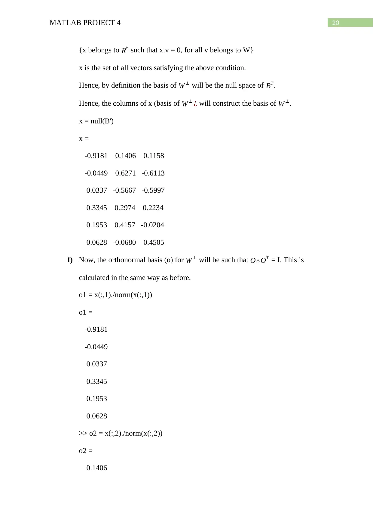
{x belongs to R6 such that x.v = 0, for all v belongs to W}
x is the set of all vectors satisfying the above condition.
Hence, by definition the basis of W⊥ will be the null space of BT .
Hence, the columns of x (basis of W ⊥ ¿ will construct the basis of W ⊥.
x = null(B')
x =
-0.9181 0.1406 0.1158
-0.0449 0.6271 -0.6113
0.0337 -0.5667 -0.5997
0.3345 0.2974 0.2234
0.1953 0.4157 -0.0204
0.0628 -0.0680 0.4505
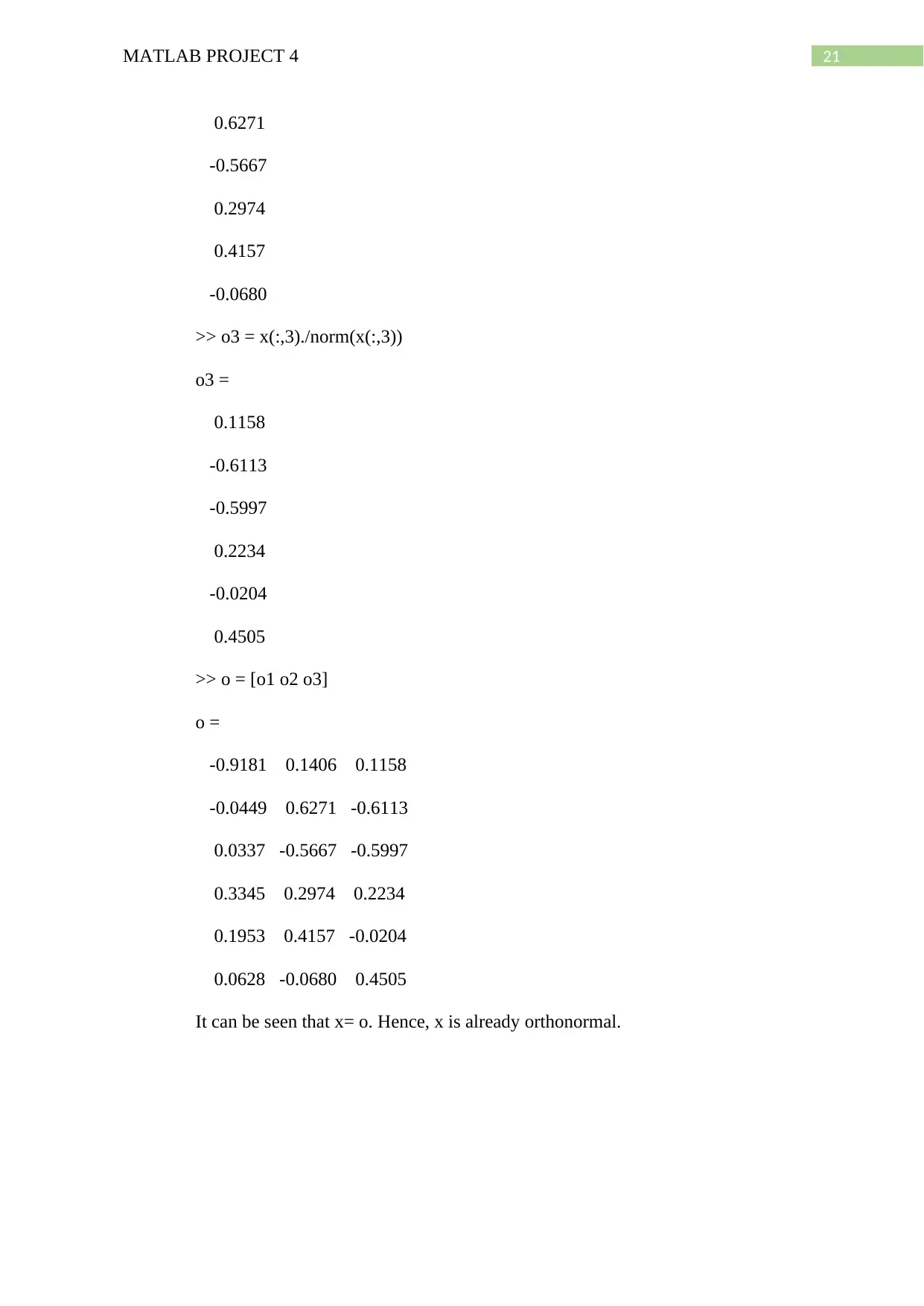
f) Now, the orthonormal basis (o) for W ⊥ will be such that O∗OT = I. This is
calculated in the same way as before.
o1 = x(:,1)./norm(x(:,1))
o1 =
-0.9181
-0.0449
0.0337
0.3345
0.1953
0.0628
>> o2 = x(:,2)./norm(x(:,2))
o2 =
0.1406
21MATLAB PROJECT 4
0.6271
-0.5667
0.2974
0.4157
-0.0680
>> o3 = x(:,3)./norm(x(:,3))
o3 =
0.1158
-0.6113
-0.5997
0.2234
-0.0204
0.4505
>> o = [o1 o2 o3]
o =
-0.9181 0.1406 0.1158
-0.0449 0.6271 -0.6113
0.0337 -0.5667 -0.5997
0.3345 0.2974 0.2234
0.1953 0.4157 -0.0204
0.0628 -0.0680 0.4505
It can be seen that x= o. Hence, x is already orthonormal.
Secure Best Marks with AI Grader
Need help grading? Try our AI Grader for instant feedback on your assignments.
22MATLAB PROJECT 4
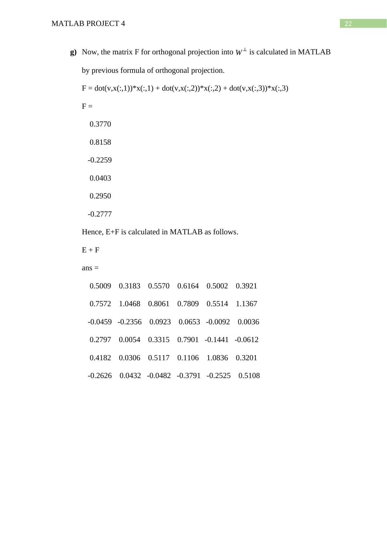
g) Now, the matrix F for orthogonal projection into W ⊥ is calculated in MATLAB
by previous formula of orthogonal projection.
F = dot(v,x(:,1))*x(:,1) + dot(v,x(:,2))*x(:,2) + dot(v,x(:,3))*x(:,3)
F =
0.3770
0.8158
-0.2259
0.0403
0.2950
-0.2777
Hence, E+F is calculated in MATLAB as follows.
E + F
ans =
0.5009 0.3183 0.5570 0.6164 0.5002 0.3921
0.7572 1.0468 0.8061 0.7809 0.5514 1.1367
-0.0459 -0.2356 0.0923 0.0653 -0.0092 0.0036
0.2797 0.0054 0.3315 0.7901 -0.1441 -0.0612
0.4182 0.0306 0.5117 0.1106 1.0836 0.3201
-0.2626 0.0432 -0.0482 -0.3791 -0.2525 0.5108

23MATLAB PROJECT 4
1 out of 24
Your All-in-One AI-Powered Toolkit for Academic Success.
+13062052269
info@desklib.com
Available 24*7 on WhatsApp / Email
![[object Object]](/_next/static/media/star-bottom.7253800d.svg)
Unlock your academic potential
© 2024 | Zucol Services PVT LTD | All rights reserved.