Group Assignment – Statistics

Running head: GROUP ASSIGNMENT – STATISTICS
Group Assignment – Statistics
Name
Course Number
Date
Faculty Name

GROUP ASSIGNMENT – STATISTICS 2
Group Assignment – Statistics
1. Frequency distribution and histogram
a) A table of frequency distribution, relative frequency distribution and percent frequency
distribution with a width of $50
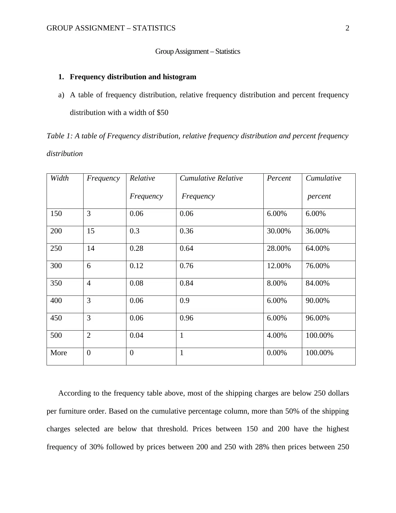
Table 1: A table of Frequency distribution, relative frequency distribution and percent frequency
distribution
Width Frequency Relative
Frequency
Cumulative Relative
Frequency
Percent Cumulative
percent
150 3 0.06 0.06 6.00% 6.00%
200 15 0.3 0.36 30.00% 36.00%
250 14 0.28 0.64 28.00% 64.00%
300 6 0.12 0.76 12.00% 76.00%
350 4 0.08 0.84 8.00% 84.00%
400 3 0.06 0.9 6.00% 90.00%
450 3 0.06 0.96 6.00% 96.00%
500 2 0.04 1 4.00% 100.00%
More 0 0 1 0.00% 100.00%
According to the frequency table above, most of the shipping charges are below 250 dollars
per furniture order. Based on the cumulative percentage column, more than 50% of the shipping
charges selected are below that threshold. Prices between 150 and 200 have the highest
frequency of 30% followed by prices between 200 and 250 with 28% then prices between 250

GROUP ASSIGNMENT – STATISTICS 3
and 300 which takes 12%. Cumulatively, 70% of the furniture shipping charges selected at
random are between 150 and 300. The width between 450 and 500 has the least frequency of 2
price values which accounts for 4%(Siegel, 2012).
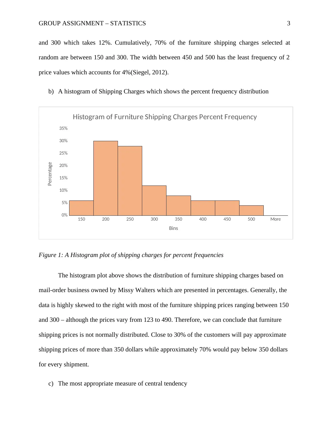
b) A histogram of Shipping Charges which shows the percent frequency distribution
150 200 250 300 350 400 450 500 More
0%
5%
10%
15%
20%
25%
30%
35%
Histogram of Furniture Shipping Charges Percent Frequency
Bins
Percentage
Figure 1: A Histogram plot of shipping charges for percent frequencies
The histogram plot above shows the distribution of furniture shipping charges based on
mail-order business owned by Missy Walters which are presented in percentages. Generally, the
data is highly skewed to the right with most of the furniture shipping prices ranging between 150
and 300 – although the prices vary from 123 to 490. Therefore, we can conclude that furniture
shipping prices is not normally distributed. Close to 30% of the customers will pay approximate
shipping prices of more than 350 dollars while approximately 70% would pay below 350 dollars
for every shipment.
c) The most appropriate measure of central tendency

GROUP ASSIGNMENT – STATISTICS 4
In such as sscenario where the data is not approximately normal, mean is not the best
measure of central tendency. Median and mode can be used to explain the best central measure,
with mode being used in discrete data where one value has a very high frequency. Median will
be the best measure of central location and quartiles to evaluate the dispersion of the values. The
median statistic is $228.5, first quartile is $182.75 and third quartile is $295.25.
2. Relationship between Demand (Y) and Unit price (X)
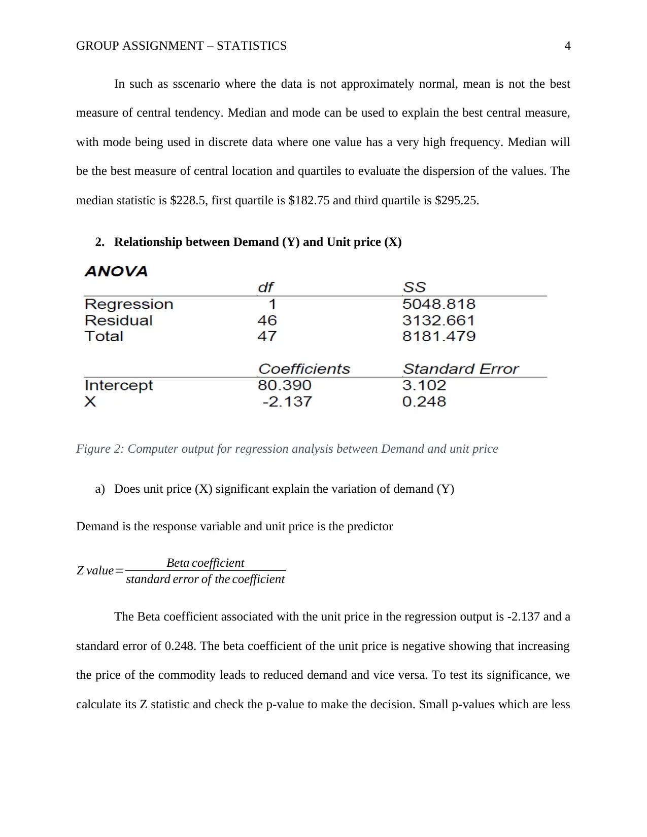
Figure 2: Computer output for regression analysis between Demand and unit price
a) Does unit price (X) significant explain the variation of demand (Y)
Demand is the response variable and unit price is the predictor
Z value= Beta coefficient
standard error of the coefficient
The Beta coefficient associated with the unit price in the regression output is -2.137 and a
standard error of 0.248. The beta coefficient of the unit price is negative showing that increasing
the price of the commodity leads to reduced demand and vice versa. To test its significance, we
calculate its Z statistic and check the p-value to make the decision. Small p-values which are less

GROUP ASSIGNMENT – STATISTICS 5
the significance level shows that the variables is a significant predictor in the model(Aiken,
West, & Pitts, 2003).
−2.137
0.248 =−8.167
The p-value associated with a Z-statistic of -8.167 is very small (<0.001)
p−value<0.001
Since the p-value is very small, the unit price is a significant predictor of demand.
Therefore, we conclude that demand and unit price are significantly related and the unit price can
be used to predict the level of demand.
b) Compute Coefficient of determination and explain its meaning
Coefficient of determination is a statistic which is used to evaluate the significance of a
model in terms of the level of variation which can be explained by the set of predictors. It ranges
between 0 and 1 and higher values symbolize a better model. This statistic is calculated using the
formula below. It mostly referred to as the R-squared statistic(Devore, 2006).
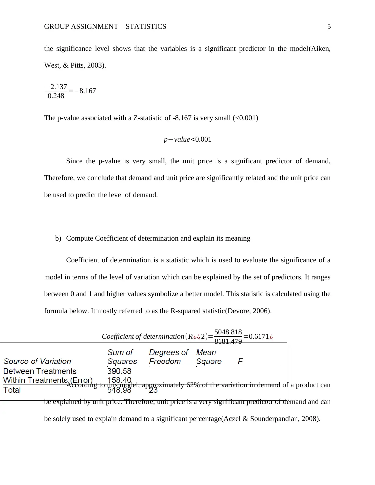
Coefficient of determination (R¿¿ 2)= 5048.818
8181.479 =0.6171¿
According to this model, approximately 62% of the variation in demand of a product can
be explained by unit price. Therefore, unit price is a very significant predictor of demand and can
be solely used to explain demand to a significant percentage(Aczel & Sounderpandian, 2008).

GROUP ASSIGNMENT – STATISTICS 6
c) Compute coefficient of correlation and explain the relationship between demand and unit
price
The coeffient is correlation is calculated by taking the square root of the R-squared statistic as
shown below.
√ 0.6171=0.786
There is a strong negative relationship between unit price and demand. We conclude that
the relationship is negative because the model coefficient associated with unit price is negative.
Therefore, as the price increases, the demand of the product reduces. This is because most people
will be willing to buy products with low prices compared with pricy products(Siegel, 2012).
3. Randomized study design with 3 treatments
Figure 3: One way ANOVA model computer output for three treatments
Degrees of freedom of thetreatments
There are three treatments and the formula of degrees of freedom is number of treatments−1
3−1=2
Degrees of freedom associated with error

GROUP ASSIGNMENT – STATISTICS 7
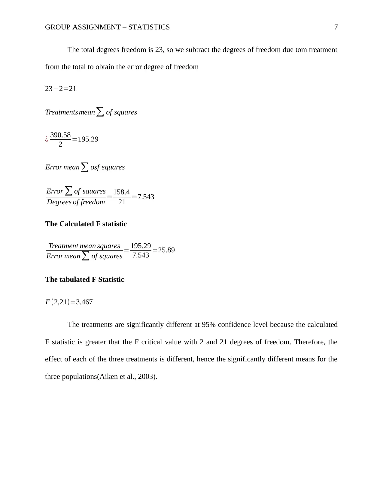
The total degrees freedom is 23, so we subtract the degrees of freedom due tom treatment
from the total to obtain the error degree of freedom
23−2=21
Treatmentsmean ∑ of squares
¿ 390.58
2 =195.29
Error mean∑ osf squares
Error ∑ of squares
Degrees of freedom =158.4
21 =7.543
The Calculated F statistic
Treatment mean squares
Error mean∑ of squares = 195.29
7.543 =25.89
The tabulated F Statistic
F (2,21)=3.467
The treatments are significantly different at 95% confidence level because the calculated
F statistic is greater that the F critical value with 2 and 21 degrees of freedom. Therefore, the
effect of each of the three treatments is different, hence the significantly different means for the
three populations(Aiken et al., 2003).

GROUP ASSIGNMENT – STATISTICS 8
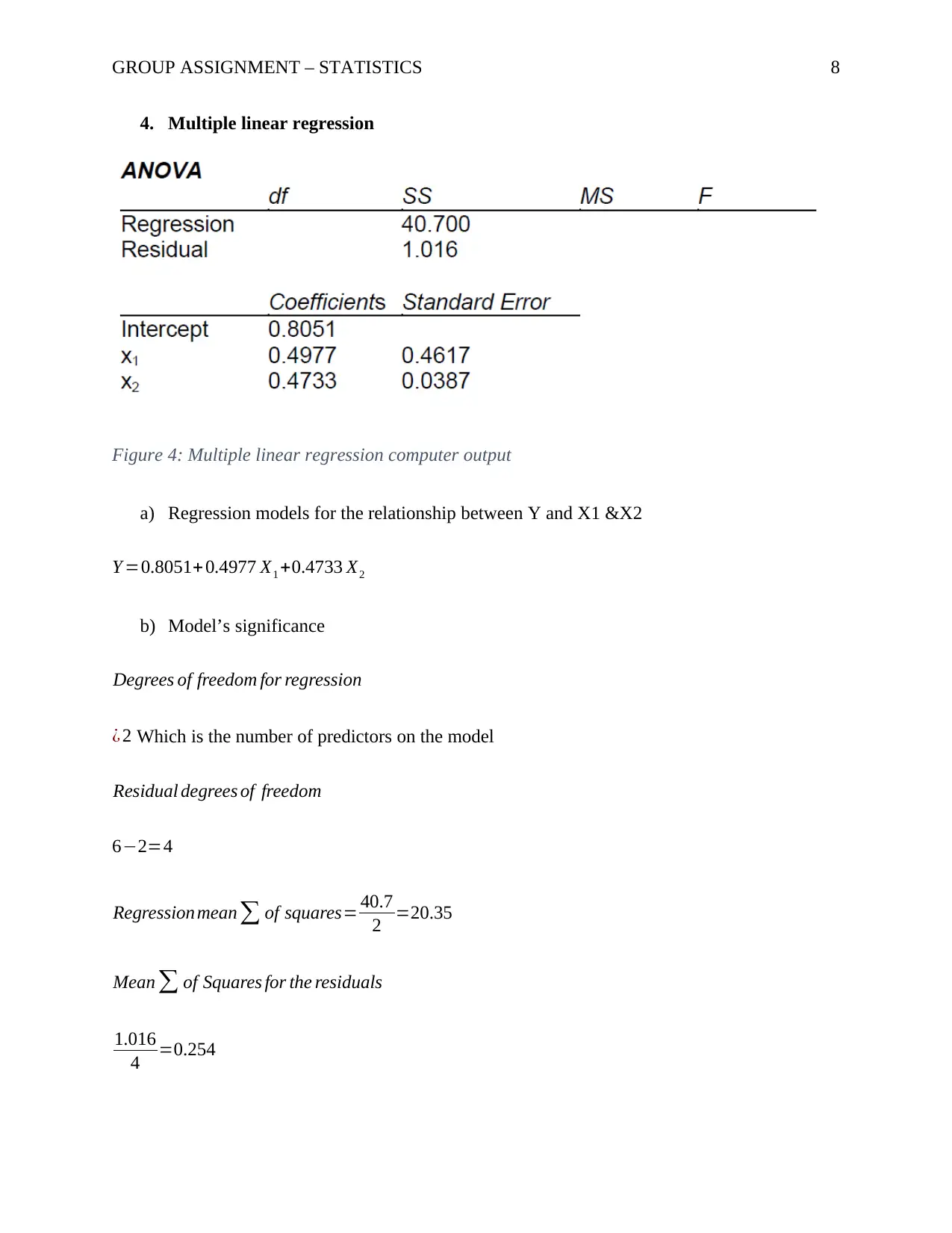
4. Multiple linear regression
Figure 4: Multiple linear regression computer output
a) Regression models for the relationship between Y and X1 &X2
Y =0.8051+ 0.4977 X1 +0.4733 X2
b) Model’s significance
Degrees of freedom for regression
¿ 2 Which is the number of predictors on the model
Residual degrees of freedom
6−2=4
Regression mean∑ of squares= 40.7
2 =20.35
Mean ∑ of Squares for the residuals
1.016
4 =0.254

GROUP ASSIGNMENT – STATISTICS 9
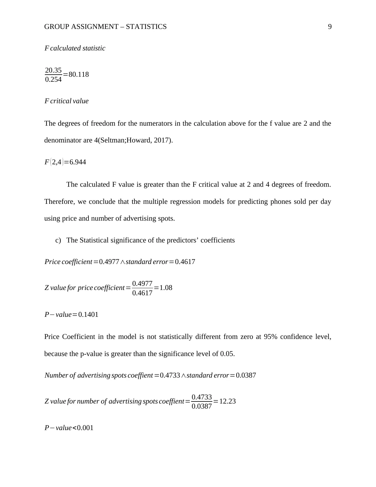
F calculated statistic
20.35
0.254 =80.118
F critical value
The degrees of freedom for the numerators in the calculation above for the f value are 2 and the
denominator are 4(Seltman;Howard, 2017).
F ( 2,4 )=6.944
The calculated F value is greater than the F critical value at 2 and 4 degrees of freedom.
Therefore, we conclude that the multiple regression models for predicting phones sold per day
using price and number of advertising spots.
c) The Statistical significance of the predictors’ coefficients
Price coefficient =0.4977∧standard error=0.4617
Z value for price coefficient= 0.4977
0.4617 =1.08
P−value=0.1401
Price Coefficient in the model is not statistically different from zero at 95% confidence level,
because the p-value is greater than the significance level of 0.05.
Number of advertising spots coeffient =0.4733∧standard error=0.0387
Z value for number of advertising spots coeffient= 0.4733
0.0387 =12.23
P−value<0.001

GROUP ASSIGNMENT – STATISTICS 10
The p-value is very small, hence the conclusion that number of advertising spots coefficient is
statistically difference from zero(Huberty, 2003).
d) Slope coefficient for number of advertising spots
Increasing the number of advertising spots by one, the number of mobile phones sold in a day
will increase by 0.4733.
e) Using the model to predict number of phones sold
10 advertisement spots and $20,000 per phone
Y =0.8051+ 0.4977(20)+0.4733(10)
¿ 15.4921
Around 16 phones shall be sold for $20,000 per phone and using10 advertising spots.

GROUP ASSIGNMENT – STATISTICS 11
References
Aczel, A. D., & Sounderpandian, J. (2008). Complete: Business Statistics. ASSOCIATION OF
BUSINESS INFORMATION …. Retrieved from http://scholar.google.com/scholar?
hl=en&btnG=Search&q=intitle:McGraw-Hill/Irwin+=%3E?#1
Aiken, L. S., West, S. G., & Pitts, S. C. (2003). Multiple Linear Regression. Handbook of
Psychology, 481–507. https://doi.org/10.1051/eas/1466005
Devore, J. (2006). Statistics for Business and Economics. The American Statistician, 60(4), 342–
343. https://doi.org/10.1198/tas.2006.s59
Huberty, C. J. (2003). Multiple correlation versus multiple regression. Educational and
Psychological Measurement, 63(2), 271–278. https://doi.org/10.1177/0013164402250990
Seltman;Howard. (2017). One-Way ANOVA. Experimental Design and Analysis, 171–190.
Retrieved from https://www.jmp.com/content/dam/jmp/documents/en/academic/learning-
library/04-one-way-anova.pdf
Siegel, A. F. (2012). Practical Business Statistics. Practical Business Statistics.
https://doi.org/10.1016/B978-0-12-385208-3.00014-6