Grouping Data into Tables using RStudio for Manufacturing Energy Consumption Survey (MECS) except the Petroleum Refining Industry
VerifiedAdded on 2022/11/23
|9
|1456
|141
AI Summary
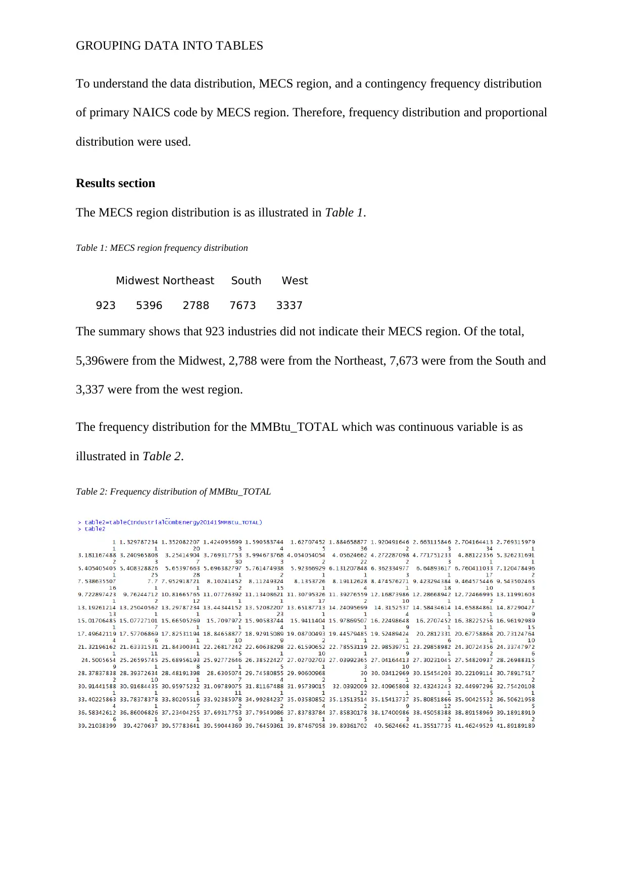
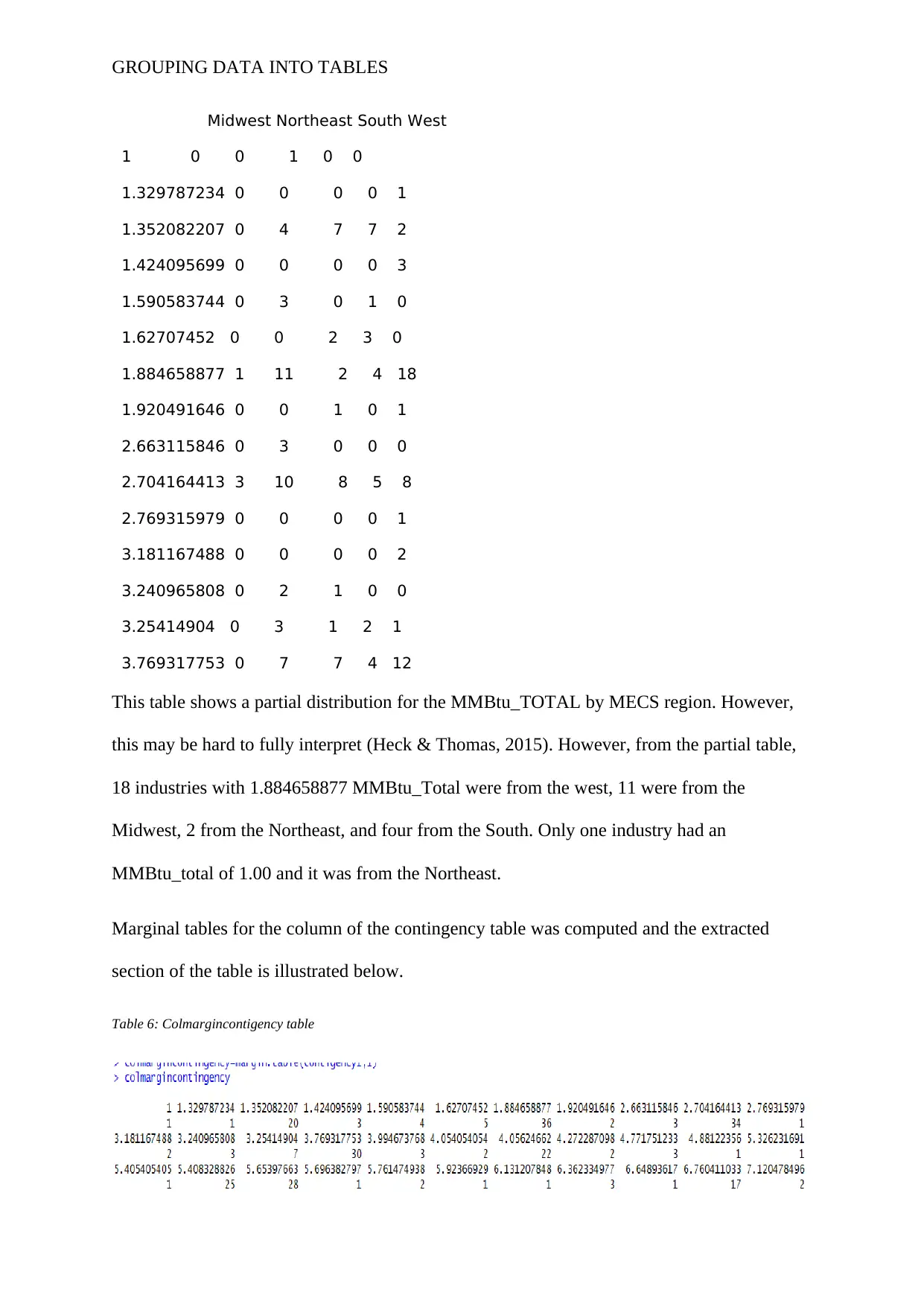
This report will highlight the distribution of the Manufacturing, Energy Consumption Survey (MECS) except the Petroleum Refining Industry by the MECS region. The data used will be from the MECS 2014 which in total had 20,117 establishments which is a good representation of the US industry. The survey data are collected as a national sample survey with information about energy consumption and expenditures and energy-related characteristics.
Contribute Materials
Your contribution can guide someone’s learning journey. Share your
documents today.
1 out of 9
Related Documents


Your All-in-One AI-Powered Toolkit for Academic Success.
+13062052269
info@desklib.com
Available 24*7 on WhatsApp / Email
![[object Object]](/_next/static/media/star-bottom.7253800d.svg)
© 2024 | Zucol Services PVT LTD | All rights reserved.