Data Analysis: Health and Wellbeing

SPSS output for a study on Health and Wellbeing including descriptive statistics of age, demographic information, equality of means of aggression, thrill seeking and risk acceptance by gender, metropolitan background status, and study mode, and chi-square test of independence for depressed and gender, depression and metropolitan background status, depression and study mode, depression and fee status, road traffic accidents as dependent variable, and obesity at third year as dependent variable.

SPSS OUTPUT
Name
Course Number
Date
Faculty Name

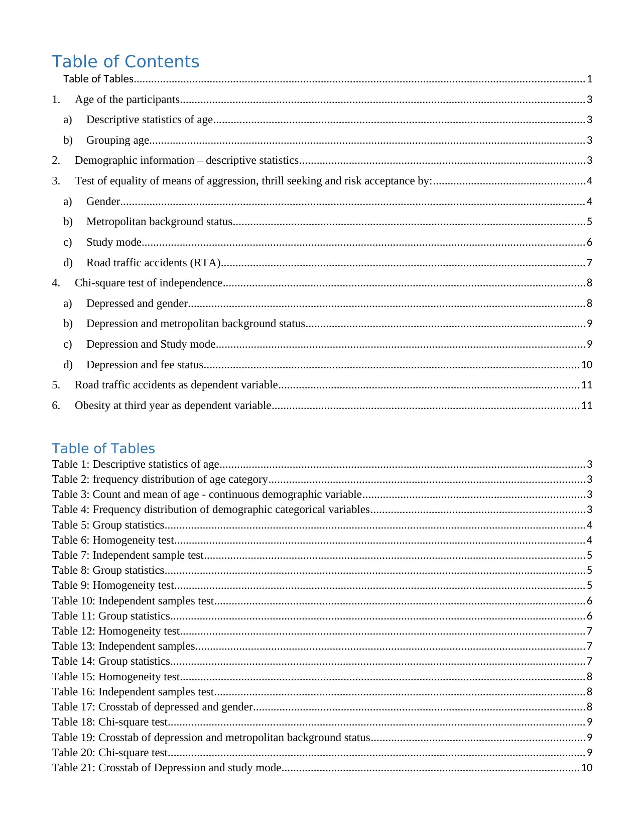
Table of Contents
Table of Tables..........................................................................................................................................................1
1. Age of the participants..........................................................................................................................................3
a) Descriptive statistics of age...............................................................................................................................3
b) Grouping age.....................................................................................................................................................3
2. Demographic information – descriptive statistics..................................................................................................3
3. Test of equality of means of aggression, thrill seeking and risk acceptance by:....................................................4
a) Gender...............................................................................................................................................................4
b) Metropolitan background status........................................................................................................................5
c) Study mode.......................................................................................................................................................6
d) Road traffic accidents (RTA)............................................................................................................................7
4. Chi-square test of independence............................................................................................................................8
a) Depressed and gender........................................................................................................................................8
b) Depression and metropolitan background status................................................................................................9
c) Depression and Study mode..............................................................................................................................9
d) Depression and fee status................................................................................................................................10
5. Road traffic accidents as dependent variable.......................................................................................................11
6. Obesity at third year as dependent variable.........................................................................................................11
Table of Tables
Table 1: Descriptive statistics of age.............................................................................................................................3
Table 2: frequency distribution of age category............................................................................................................3
Table 3: Count and mean of age - continuous demographic variable............................................................................3
Table 4: Frequency distribution of demographic categorical variables.........................................................................3
Table 5: Group statistics................................................................................................................................................4
Table 6: Homogeneity test............................................................................................................................................4
Table 7: Independent sample test..................................................................................................................................5
Table 8: Group statistics................................................................................................................................................5
Table 9: Homogeneity test............................................................................................................................................5
Table 10: Independent samples test...............................................................................................................................6
Table 11: Group statistics..............................................................................................................................................6
Table 12: Homogeneity test..........................................................................................................................................7
Table 13: Independent samples.....................................................................................................................................7
Table 14: Group statistics..............................................................................................................................................7
Table 15: Homogeneity test..........................................................................................................................................8
Table 16: Independent samples test...............................................................................................................................8
Table 17: Crosstab of depressed and gender.................................................................................................................8
Table 18: Chi-square test...............................................................................................................................................9
Table 19: Crosstab of depression and metropolitan background status.........................................................................9
Table 20: Chi-square test...............................................................................................................................................9
Table 21: Crosstab of Depression and study mode......................................................................................................10

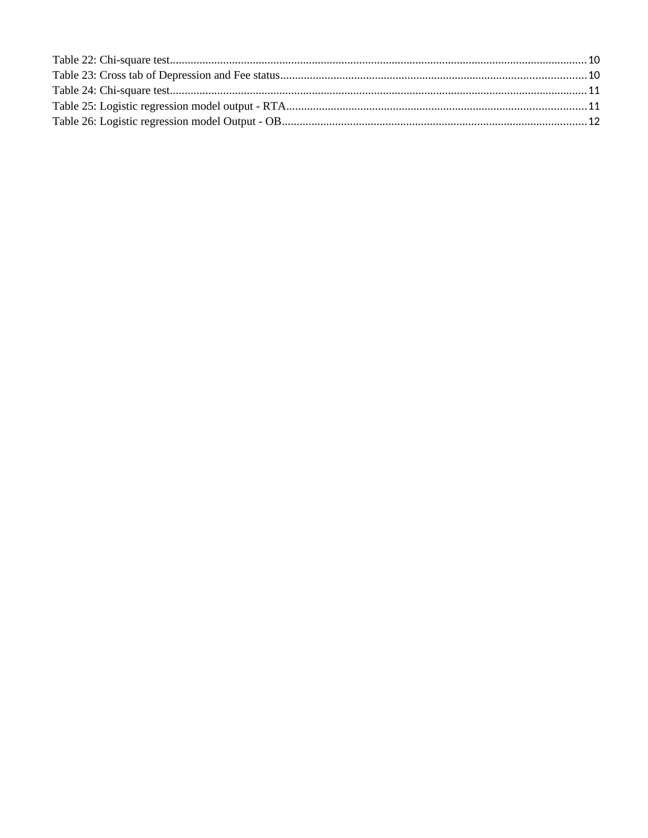
Table 22: Chi-square test.............................................................................................................................................10
Table 23: Cross tab of Depression and Fee status.......................................................................................................10
Table 24: Chi-square test.............................................................................................................................................11
Table 25: Logistic regression model output - RTA.....................................................................................................11
Table 26: Logistic regression model Output - OB.......................................................................................................12

Data Analysis: Health and Wellbeing
1. Age of the participants
a) Descriptive statistics of age
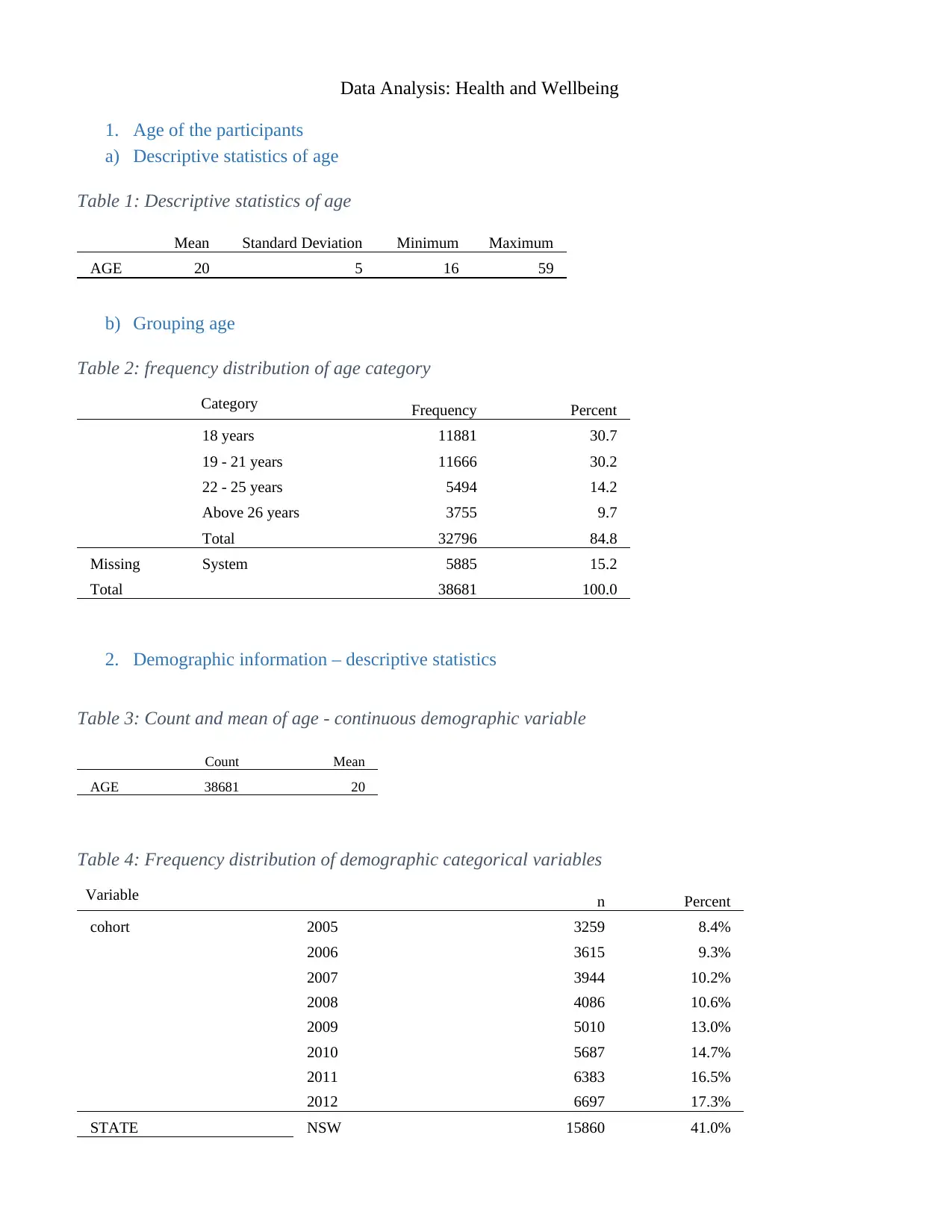
Table 1: Descriptive statistics of age
Mean Standard Deviation Minimum Maximum
AGE 20 5 16 59
b) Grouping age
Table 2: frequency distribution of age category
Category Frequency Percent
18 years 11881 30.7
19 - 21 years 11666 30.2
22 - 25 years 5494 14.2
Above 26 years 3755 9.7
Total 32796 84.8
Missing System 5885 15.2
Total 38681 100.0
2. Demographic information – descriptive statistics
Table 3: Count and mean of age - continuous demographic variable
Count Mean
AGE 38681 20
Table 4: Frequency distribution of demographic categorical variables
Variable n Percent
cohort 2005 3259 8.4%
2006 3615 9.3%
2007 3944 10.2%
2008 4086 10.6%
2009 5010 13.0%
2010 5687 14.7%
2011 6383 16.5%
2012 6697 17.3%
STATE NSW 15860 41.0%

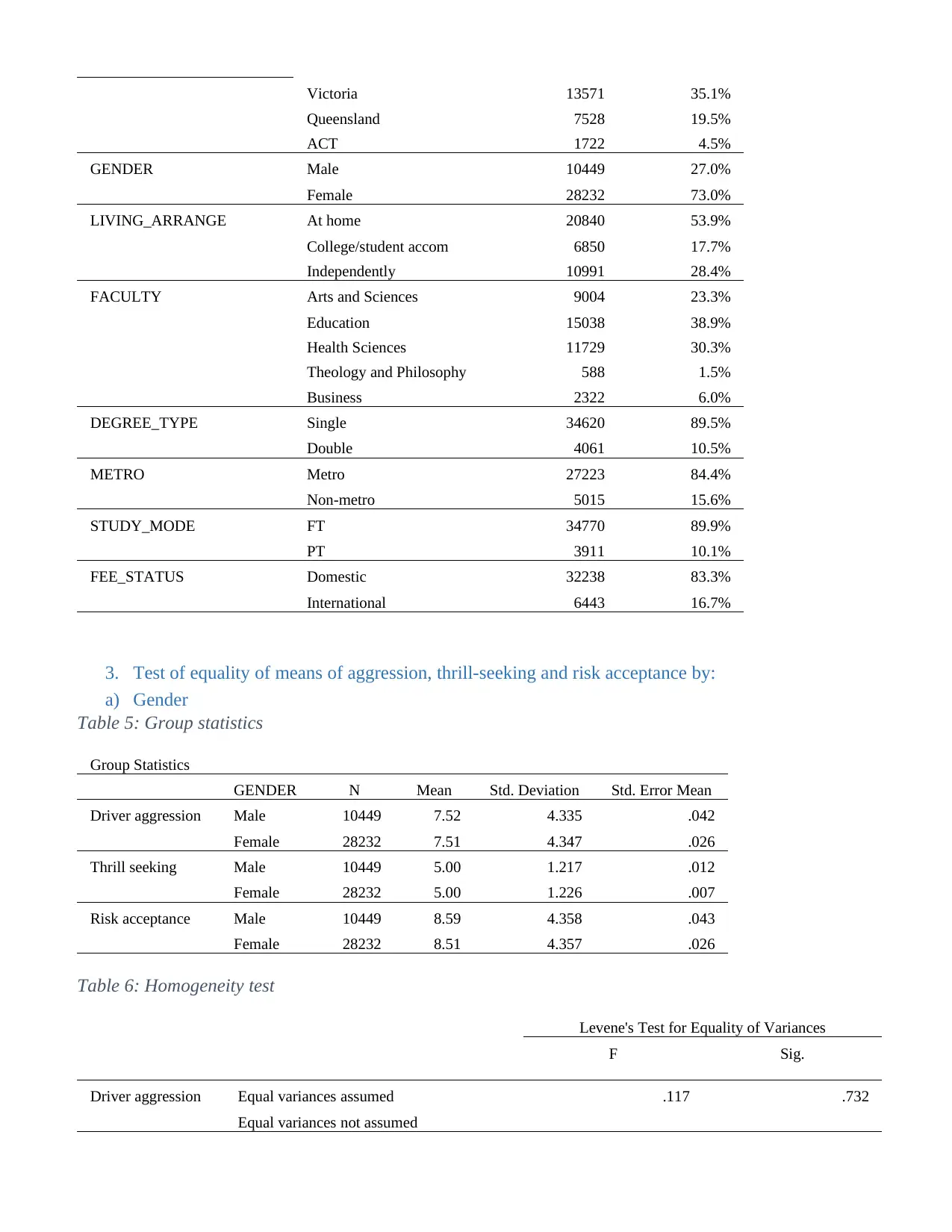
Victoria 13571 35.1%
Queensland 7528 19.5%
ACT 1722 4.5%
GENDER Male 10449 27.0%
Female 28232 73.0%
LIVING_ARRANGE At home 20840 53.9%
College/student accom 6850 17.7%
Independently 10991 28.4%
FACULTY Arts and Sciences 9004 23.3%
Education 15038 38.9%
Health Sciences 11729 30.3%
Theology and Philosophy 588 1.5%
Business 2322 6.0%
DEGREE_TYPE Single 34620 89.5%
Double 4061 10.5%
METRO Metro 27223 84.4%
Non-metro 5015 15.6%
STUDY_MODE FT 34770 89.9%
PT 3911 10.1%
FEE_STATUS Domestic 32238 83.3%
International 6443 16.7%
3. Test of equality of means of aggression, thrill-seeking and risk acceptance by:
a) Gender
Table 5: Group statistics
Group Statistics
GENDER N Mean Std. Deviation Std. Error Mean
Driver aggression Male 10449 7.52 4.335 .042
Female 28232 7.51 4.347 .026
Thrill seeking Male 10449 5.00 1.217 .012
Female 28232 5.00 1.226 .007
Risk acceptance Male 10449 8.59 4.358 .043
Female 28232 8.51 4.357 .026
Table 6: Homogeneity test
Levene's Test for Equality of Variances
F Sig.
Driver aggression Equal variances assumed .117 .732
Equal variances not assumed

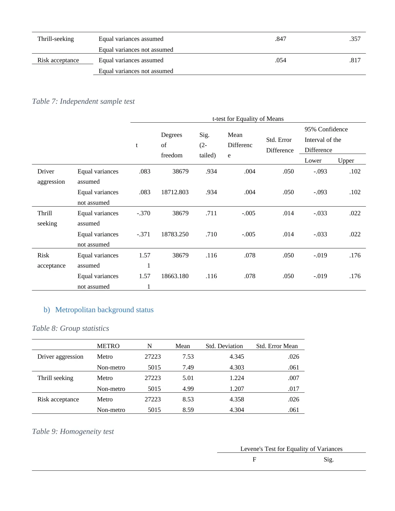
Thrill-seeking Equal variances assumed .847 .357
Equal variances not assumed
Risk acceptance Equal variances assumed .054 .817
Equal variances not assumed
Table 7: Independent sample test
t-test for Equality of Means
t
Degrees
of
freedom
Sig.
(2-
tailed)
Mean
Differenc
e
Std. Error
Difference
95% Confidence
Interval of the
Difference
Lower Upper
Driver
aggression
Equal variances
assumed
.083 38679 .934 .004 .050 -.093 .102
Equal variances
not assumed
.083 18712.803 .934 .004 .050 -.093 .102
Thrill
seeking
Equal variances
assumed
-.370 38679 .711 -.005 .014 -.033 .022
Equal variances
not assumed
-.371 18783.250 .710 -.005 .014 -.033 .022
Risk
acceptance
Equal variances
assumed
1.57
1
38679 .116 .078 .050 -.019 .176
Equal variances
not assumed
1.57
1
18663.180 .116 .078 .050 -.019 .176
b) Metropolitan background status
Table 8: Group statistics
METRO N Mean Std. Deviation Std. Error Mean
Driver aggression Metro 27223 7.53 4.345 .026
Non-metro 5015 7.49 4.303 .061
Thrill seeking Metro 27223 5.01 1.224 .007
Non-metro 5015 4.99 1.207 .017
Risk acceptance Metro 27223 8.53 4.358 .026
Non-metro 5015 8.59 4.304 .061
Table 9: Homogeneity test
Levene's Test for Equality of Variances
F Sig.

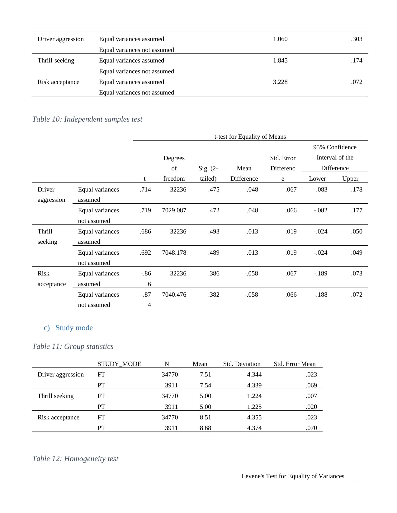
Driver aggression Equal variances assumed 1.060 .303
Equal variances not assumed
Thrill-seeking Equal variances assumed 1.845 .174
Equal variances not assumed
Risk acceptance Equal variances assumed 3.228 .072
Equal variances not assumed
Table 10: Independent samples test
t-test for Equality of Means
t
Degrees
of
freedom
Sig. (2-
tailed)
Mean
Difference
Std. Error
Differenc
e
95% Confidence
Interval of the
Difference
Lower Upper
Driver
aggression
Equal variances
assumed
.714 32236 .475 .048 .067 -.083 .178
Equal variances
not assumed
.719 7029.087 .472 .048 .066 -.082 .177
Thrill
seeking
Equal variances
assumed
.686 32236 .493 .013 .019 -.024 .050
Equal variances
not assumed
.692 7048.178 .489 .013 .019 -.024 .049
Risk
acceptance
Equal variances
assumed
-.86
6
32236 .386 -.058 .067 -.189 .073
Equal variances
not assumed
-.87
4
7040.476 .382 -.058 .066 -.188 .072
c) Study mode
Table 11: Group statistics
STUDY_MODE N Mean Std. Deviation Std. Error Mean
Driver aggression FT 34770 7.51 4.344 .023
PT 3911 7.54 4.339 .069
Thrill seeking FT 34770 5.00 1.224 .007
PT 3911 5.00 1.225 .020
Risk acceptance FT 34770 8.51 4.355 .023
PT 3911 8.68 4.374 .070
Table 12: Homogeneity test
Levene's Test for Equality of Variances

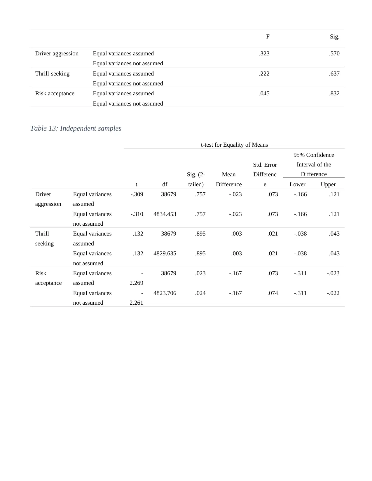
F Sig.
Driver aggression Equal variances assumed .323 .570
Equal variances not assumed
Thrill-seeking Equal variances assumed .222 .637
Equal variances not assumed
Risk acceptance Equal variances assumed .045 .832
Equal variances not assumed
Table 13: Independent samples
t-test for Equality of Means
t df
Sig. (2-
tailed)
Mean
Difference
Std. Error
Differenc
e
95% Confidence
Interval of the
Difference
Lower Upper
Driver
aggression
Equal variances
assumed
-.309 38679 .757 -.023 .073 -.166 .121
Equal variances
not assumed
-.310 4834.453 .757 -.023 .073 -.166 .121
Thrill
seeking
Equal variances
assumed
.132 38679 .895 .003 .021 -.038 .043
Equal variances
not assumed
.132 4829.635 .895 .003 .021 -.038 .043
Risk
acceptance
Equal variances
assumed
-
2.269
38679 .023 -.167 .073 -.311 -.023
Equal variances
not assumed
-
2.261
4823.706 .024 -.167 .074 -.311 -.022

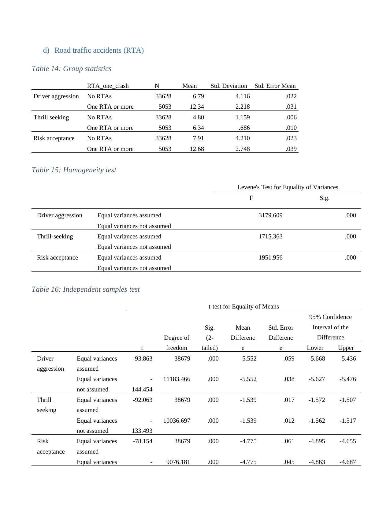
d) Road traffic accidents (RTA)
Table 14: Group statistics
RTA_one_crash N Mean Std. Deviation Std. Error Mean
Driver aggression No RTAs 33628 6.79 4.116 .022
One RTA or more 5053 12.34 2.218 .031
Thrill seeking No RTAs 33628 4.80 1.159 .006
One RTA or more 5053 6.34 .686 .010
Risk acceptance No RTAs 33628 7.91 4.210 .023
One RTA or more 5053 12.68 2.748 .039
Table 15: Homogeneity test
Levene's Test for Equality of Variances
F Sig.
Driver aggression Equal variances assumed 3179.609 .000
Equal variances not assumed
Thrill-seeking Equal variances assumed 1715.363 .000
Equal variances not assumed
Risk acceptance Equal variances assumed 1951.956 .000
Equal variances not assumed
Table 16: Independent samples test
t-test for Equality of Means
t
Degree of
freedom
Sig.
(2-
tailed)
Mean
Differenc
e
Std. Error
Differenc
e
95% Confidence
Interval of the
Difference
Lower Upper
Driver
aggression
Equal variances
assumed
-93.863 38679 .000 -5.552 .059 -5.668 -5.436
Equal variances
not assumed
-
144.454
11183.466 .000 -5.552 .038 -5.627 -5.476
Thrill
seeking
Equal variances
assumed
-92.063 38679 .000 -1.539 .017 -1.572 -1.507
Equal variances
not assumed
-
133.493
10036.697 .000 -1.539 .012 -1.562 -1.517
Risk
acceptance
Equal variances
assumed
-78.154 38679 .000 -4.775 .061 -4.895 -4.655
Equal variances - 9076.181 .000 -4.775 .045 -4.863 -4.687

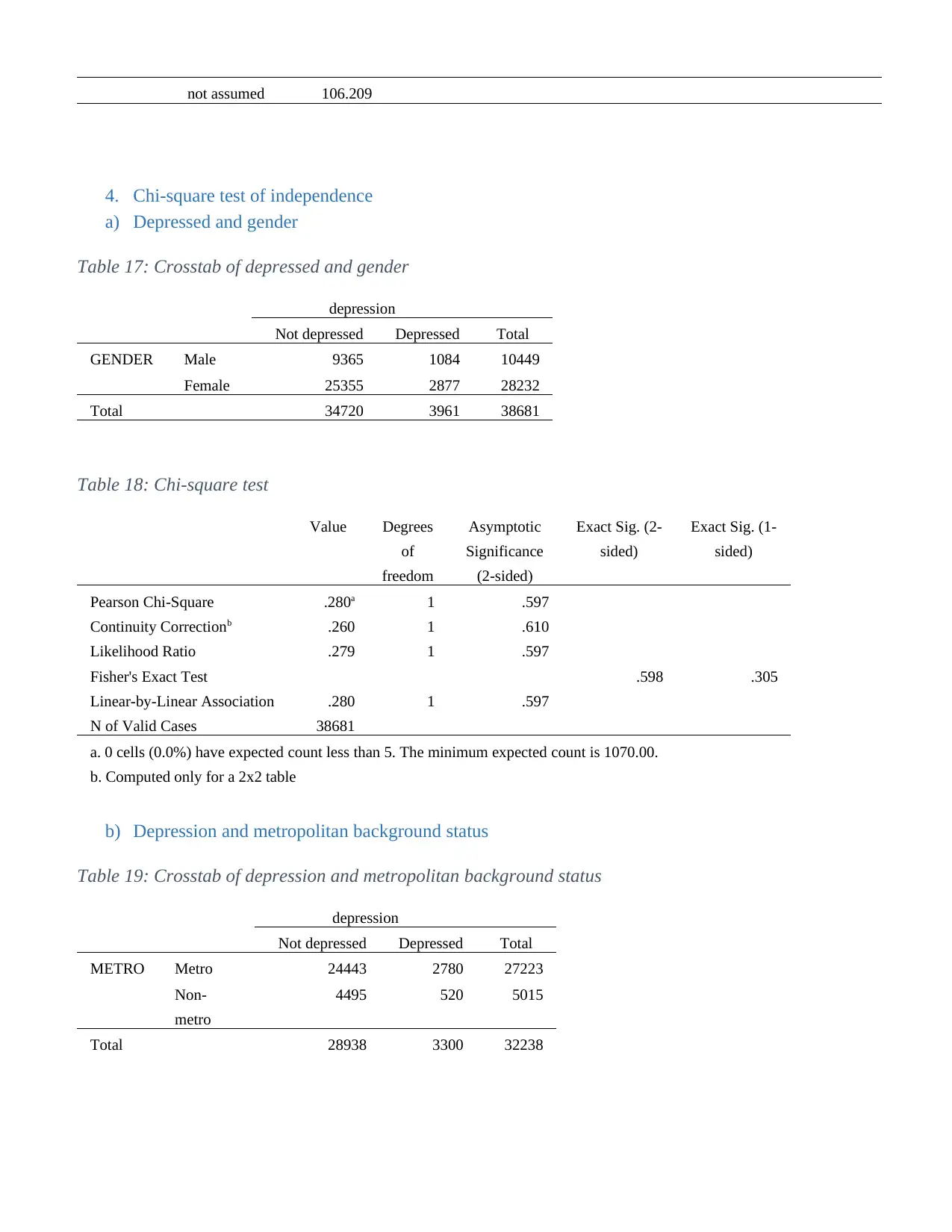
not assumed 106.209
4. Chi-square test of independence
a) Depressed and gender
Table 17: Crosstab of depressed and gender
depression
Not depressed Depressed Total
GENDER Male 9365 1084 10449
Female 25355 2877 28232
Total 34720 3961 38681
Table 18: Chi-square test
Value Degrees
of
freedom
Asymptotic
Significance
(2-sided)
Exact Sig. (2-
sided)
Exact Sig. (1-
sided)
Pearson Chi-Square .280a 1 .597
Continuity Correctionb .260 1 .610
Likelihood Ratio .279 1 .597
Fisher's Exact Test .598 .305
Linear-by-Linear Association .280 1 .597
N of Valid Cases 38681
a. 0 cells (0.0%) have expected count less than 5. The minimum expected count is 1070.00.
b. Computed only for a 2x2 table
b) Depression and metropolitan background status
Table 19: Crosstab of depression and metropolitan background status
depression
Not depressed Depressed Total
METRO Metro 24443 2780 27223
Non-
metro
4495 520 5015
Total 28938 3300 32238

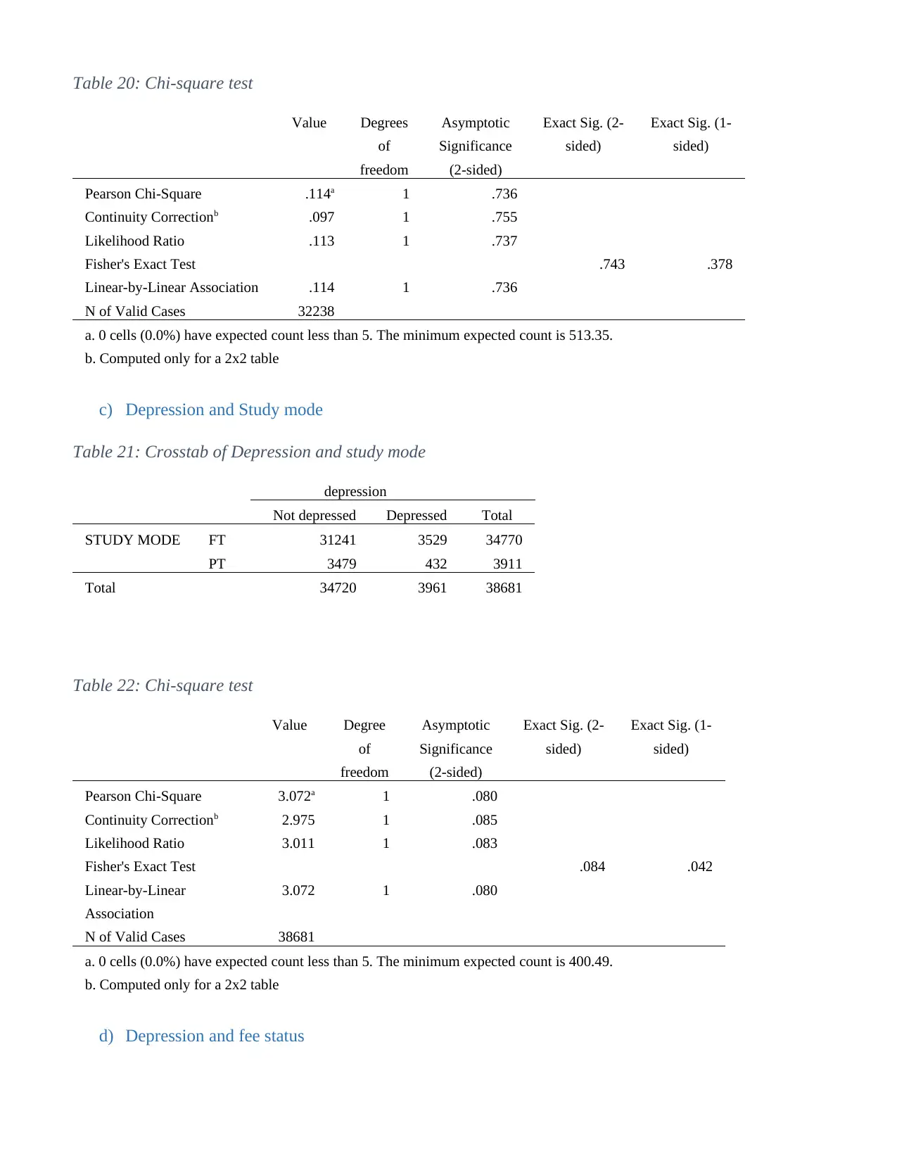
Table 20: Chi-square test
Value Degrees
of
freedom
Asymptotic
Significance
(2-sided)
Exact Sig. (2-
sided)
Exact Sig. (1-
sided)
Pearson Chi-Square .114a 1 .736
Continuity Correctionb .097 1 .755
Likelihood Ratio .113 1 .737
Fisher's Exact Test .743 .378
Linear-by-Linear Association .114 1 .736
N of Valid Cases 32238
a. 0 cells (0.0%) have expected count less than 5. The minimum expected count is 513.35.
b. Computed only for a 2x2 table
c) Depression and Study mode
Table 21: Crosstab of Depression and study mode
depression
Not depressed Depressed Total
STUDY MODE FT 31241 3529 34770
PT 3479 432 3911
Total 34720 3961 38681
Table 22: Chi-square test
Value Degree
of
freedom
Asymptotic
Significance
(2-sided)
Exact Sig. (2-
sided)
Exact Sig. (1-
sided)
Pearson Chi-Square 3.072a 1 .080
Continuity Correctionb 2.975 1 .085
Likelihood Ratio 3.011 1 .083
Fisher's Exact Test .084 .042
Linear-by-Linear
Association
3.072 1 .080
N of Valid Cases 38681
a. 0 cells (0.0%) have expected count less than 5. The minimum expected count is 400.49.
b. Computed only for a 2x2 table
d) Depression and fee status

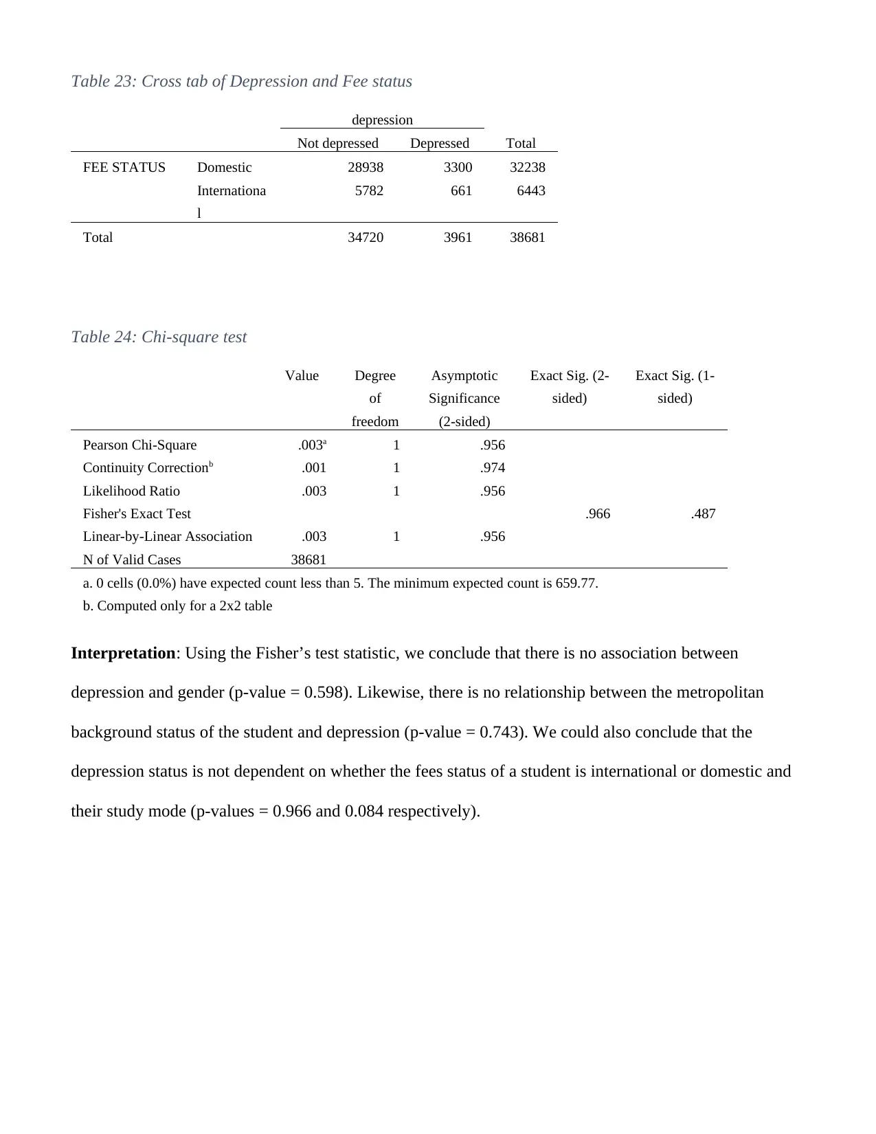
Table 23: Cross tab of Depression and Fee status
depression
TotalNot depressed Depressed
FEE STATUS Domestic 28938 3300 32238
Internationa
l
5782 661 6443
Total 34720 3961 38681
Table 24: Chi-square test
Value Degree
of
freedom
Asymptotic
Significance
(2-sided)
Exact Sig. (2-
sided)
Exact Sig. (1-
sided)
Pearson Chi-Square .003a 1 .956
Continuity Correctionb .001 1 .974
Likelihood Ratio .003 1 .956
Fisher's Exact Test .966 .487
Linear-by-Linear Association .003 1 .956
N of Valid Cases 38681
a. 0 cells (0.0%) have expected count less than 5. The minimum expected count is 659.77.
b. Computed only for a 2x2 table
Interpretation: Using the Fisher’s test statistic, we conclude that there is no association between
depression and gender (p-value = 0.598). Likewise, there is no relationship between the metropolitan
background status of the student and depression (p-value = 0.743). We could also conclude that the
depression status is not dependent on whether the fees status of a student is international or domestic and
their study mode (p-values = 0.966 and 0.084 respectively).

Logistic regression
5. Road traffic accidents as dependent variable
Table 25: Logistic regression model output - RTA
B S.E. Wald df Sig. Exp(B)
95% C.I.for
EXP(B)
Lower Upper
Demographics
Age category Ref Ref 288.182 3 .000
Age category(1) 1.176 .097 146.595 1 .000 3.241 2.680 3.921
Age category(2) .562 .097 33.522 1 .000 1.754 1.450 2.122
Age category(3) .043 .106 .166 1 .684 1.044 .848 1.285
GENDER -.620 .056 121.164 1 .000 .538 .482 .601
LIVING_ARRANGE Ref Ref 2.068 2 .356
LIVING_ARRANGE(1) -.095 .066 2.059 1 .151 .910 .799 1.035
LIVING_ARRANGE(2) -.038 .084 .204 1 .652 .963 .816 1.136
FEE_STATUS .535 .082 42.517 1 .000 1.707 1.454 2.005
Driving
Distance driving -.058 .052 1.210 1 .271 .944 .852 1.046
Behaviour
Driver aggression .632 .026 594.084 1 .000 1.881 1.788 1.979
thrill .513 .085 36.313 1 .000 1.671 1.414 1.975
Risk acceptance .608 .010 3443.489 1 .000 1.838 1.801 1.875
Constant -18.041 .372 2346.685 1 .000 .000
a. Variable(s) entered on step 1: driver aggression, thrill, risk acceptance
Living arrangements interpretation: In general, living arrangement is not a significant predictor of
whether a student has ever been involved in a road accident or not. This is because the p-values for all the
generated dummy variables generated are greater than the significance level (0.05). Further, students living
in college or other student residential areas had 9% less chance of having been involved in a road accident.
Similarly, students living independently had 3.7% less chance of having experienced road accident.
Effect of the predictors: Age, fee status, driver aggression, thrill-seeking and risk acceptance is associated
with increased odds of having experienced road accidents. However, gender, living arrangements and

driving distance are associated with reduced odds. Being a female is associated with 46.2% fewer odds of
having experienced a road traffic accident.
6. Obesity at their third year as the dependent variable
Table 26: Logistic regression model Output - OB
B S.E. Wald df Sig. Exp(B) 95% C.I.for
EXP(B)
Lower Upper
Demographic
Age category 163.151 3 .000
Age category(1) .693 .073 90.369 1 .000 1.999 1.733 2.306
Age category(2) .344 .074 21.649 1 .000 1.410 1.220 1.630
Age category(3) .098 .081 1.459 1 .227 1.103 .941 1.294
GENDER -.376 .042 81.220 1 .000 .686 .633 .745
LIVING_ARRANGE 17.581 2 .000
LIVING_ARRANGE(1) -.127 .047 7.135 1 .008 .881 .803 .967
LIVING_ARRANGE(2) .072 .059 1.495 1 .221 1.075 .957 1.207
Baseline characteristics
Obese/Overweight at
baseline
-.039 .039 .953 1 .329 .962 .891 1.040
depression 2.683 .061 1946.773 1 .000 14.635 12.990 16.487
Parental factors
Parents education -2.571 .071 1321.354 1 .000 .076 .067 .088
Parents Obese/Overweight 2.026 .177 130.630 1 .000 7.581 5.356 10.730
Constant -3.294 .192 293.400 1 .000 .037
a. Variable(s) entered on step 1: Parents education, Parents Obese/Overweight.
Living arrangements: The students living arrangements were associated with a lower odds ratio for
students living in the college or other student accommodation and higher odds for those living
independently. Generally, the student accommodation is a significant predictor of the being obese in their
third year of college.

Effect of Predictors on the prediction: Age, depression, and parents status of obesity is associated with
higher odds of being obese. On the other side, gender, living arrangement, obesity status at baseline, and
parents’ education are associated with lower odds of obesity.