Analysis of Heat Transfer in a Fin using Finite Difference Method
Added on 2023-06-11
8 Pages2287 Words414 Views
Introduction
Heat energy is related to the temperature of matter. For a given material and mass, thermal
energy depend upon the temperature. Due to temperature difference maintain between two
bodies then the heat transfer takes place from higher body to lower body based on law of
thermodynamic. Heat always flow from hot body to cold body. Heat is represented by symbol
Q, and its SI unit is Joule (J). The rate of heat transfer is determined in watts (W), equal to
joules per second.
Hear transfer is energy in transit, which occurs as a result of a temperature gradient or
difference. This temperature difference is thought of as a driving force that causes heat to
flow. Heat transfer occurs by three basic mechanisms or modes:
• Conduction or Diffusion
• Convection
• Radiation
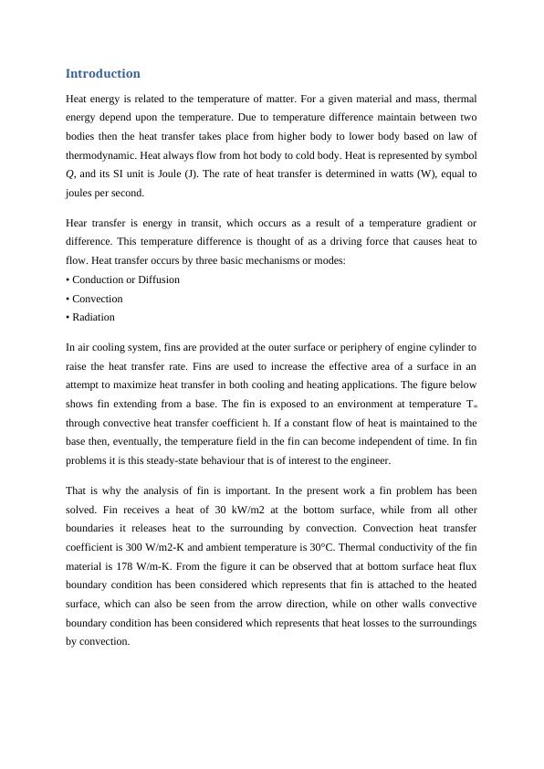
In air cooling system, fins are provided at the outer surface or periphery of engine cylinder to
raise the heat transfer rate. Fins are used to increase the effective area of a surface in an
attempt to maximize heat transfer in both cooling and heating applications. The figure below
shows fin extending from a base. The fin is exposed to an environment at temperature T∞
through convective heat transfer coefficient h. If a constant flow of heat is maintained to the
base then, eventually, the temperature field in the fin can become independent of time. In fin
problems it is this steady-state behaviour that is of interest to the engineer.
That is why the analysis of fin is important. In the present work a fin problem has been
solved. Fin receives a heat of 30 kW/m2 at the bottom surface, while from all other
boundaries it releases heat to the surrounding by convection. Convection heat transfer
coefficient is 300 W/m2-K and ambient temperature is 30°C. Thermal conductivity of the fin
material is 178 W/m-K. From the figure it can be observed that at bottom surface heat flux
boundary condition has been considered which represents that fin is attached to the heated
surface, which can also be seen from the arrow direction, while on other walls convective
boundary condition has been considered which represents that heat losses to the surroundings
by convection.
Heat energy is related to the temperature of matter. For a given material and mass, thermal
energy depend upon the temperature. Due to temperature difference maintain between two
bodies then the heat transfer takes place from higher body to lower body based on law of
thermodynamic. Heat always flow from hot body to cold body. Heat is represented by symbol
Q, and its SI unit is Joule (J). The rate of heat transfer is determined in watts (W), equal to
joules per second.
Hear transfer is energy in transit, which occurs as a result of a temperature gradient or
difference. This temperature difference is thought of as a driving force that causes heat to
flow. Heat transfer occurs by three basic mechanisms or modes:
• Conduction or Diffusion
• Convection
• Radiation
In air cooling system, fins are provided at the outer surface or periphery of engine cylinder to
raise the heat transfer rate. Fins are used to increase the effective area of a surface in an
attempt to maximize heat transfer in both cooling and heating applications. The figure below
shows fin extending from a base. The fin is exposed to an environment at temperature T∞
through convective heat transfer coefficient h. If a constant flow of heat is maintained to the
base then, eventually, the temperature field in the fin can become independent of time. In fin
problems it is this steady-state behaviour that is of interest to the engineer.
That is why the analysis of fin is important. In the present work a fin problem has been
solved. Fin receives a heat of 30 kW/m2 at the bottom surface, while from all other
boundaries it releases heat to the surrounding by convection. Convection heat transfer
coefficient is 300 W/m2-K and ambient temperature is 30°C. Thermal conductivity of the fin
material is 178 W/m-K. From the figure it can be observed that at bottom surface heat flux
boundary condition has been considered which represents that fin is attached to the heated
surface, which can also be seen from the arrow direction, while on other walls convective
boundary condition has been considered which represents that heat losses to the surroundings
by convection.
Two-dimensional heat conduction equation governs the present problem, because in present
case a solid fin has been considered. As we know in solid body heat transfer by conduction
dominates over heat transfer by convection and radiation. So the two-dimensional heat
conduction equation will govern the physical problem,
∂2 T
∂ x2 + ∂2 T
∂ y2 =0
Methodology:
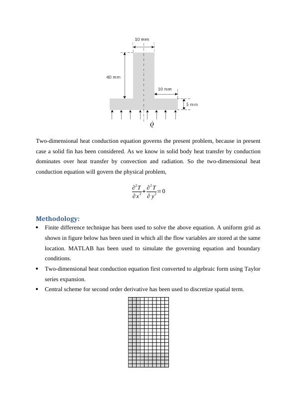
Finite difference technique has been used to solve the above equation. A uniform grid as
shown in figure below has been used in which all the flow variables are stored at the same
location. MATLAB has been used to simulate the governing equation and boundary
conditions.
Two-dimensional heat conduction equation first converted to algebraic form using Taylor
series expansion.
Central scheme for second order derivative has been used to discretize spatial term.
case a solid fin has been considered. As we know in solid body heat transfer by conduction
dominates over heat transfer by convection and radiation. So the two-dimensional heat
conduction equation will govern the physical problem,
∂2 T
∂ x2 + ∂2 T
∂ y2 =0
Methodology:
Finite difference technique has been used to solve the above equation. A uniform grid as
shown in figure below has been used in which all the flow variables are stored at the same
location. MATLAB has been used to simulate the governing equation and boundary
conditions.
Two-dimensional heat conduction equation first converted to algebraic form using Taylor
series expansion.
Central scheme for second order derivative has been used to discretize spatial term.
Boundary conditions: At the symmetry boundary condition (B2), insulated boundary
condition is applied, as no heat transfer is taking place from the symmetry wall. At B3, B4,
B6 and B7, convective boundary condition is applied. At B5 constant heat flux boundary
condition is applied.
Types of boundary condition
Dirichlet Condition or constant temperature boundary condition
Values of dependent parameter at the boundaries are defined. In the above shown problem
there is no wall on which we can consider this boundary condition. But it can be represented
as
T = T1 at y = 0 for all x values (0 ≤ x ≤ L)
T = T2 at y = H for all x values (0 ≤ x ≤ L)
Neumann Condition or insulated boundary condition
Derivative of the dependent parameter is given as a constant or as a function of the
independent variable on the boundaries.
In the above problem we can cosider this type boundary condition on the symmetry wall.
∂T
∂ x =0 At x = 0 for all y values (0 ≤ y ≤ L)
Convective type boundary condition
Derivative of the dependent variable is given as a function of the dependent variable on the
boundary.
−k ∂T
∂ x =h ( T −T∞ )
Discretize equation:
a. At B2:
∂ T
∂ x =0
Tn(1,j)=T(2,j)
b. At B5:
q=−k ∂ T
∂ x
Tn(i,1)=T(i,2)+(q*dy/k)
c. At B4:
End of preview
Want to access all the pages? Upload your documents or become a member.
Related Documents
Finite Difference Method for Two-Dimensional Heat Transfer Analysislg...
|8
|1673
|248
Heat Transfer: Analysis of Fin Configuration for Efficient Coolinglg...
|18
|3950
|33
CFD Analysis for Heat Transfer in Finslg...
|21
|2668
|323
Case Study on CFD Heat Transfer from Finslg...
|21
|2757
|52
Constant conductivity and No Heat Generation Assignment 2022lg...
|18
|1411
|34
Computational Fluid Dynamicslg...
|21
|3627
|54