Regression Analysis of Sales Data

This assignment focuses on performing a multiple linear regression analysis to predict sales based on several independent variables. It involves calculating the regression equation, examining the significance of individual predictor variables through p-values, and interpreting the coefficients' impact on sales. The task also includes predicting sales for specific values of the independent variables.

Student name: Student number:
Subject code:
Subject name:
Assignment
Due date:
Return date:
Submission method options
Alternative submission method
1

Student name: Student number:
Statement of academic integrity
2

Student name: Student number:
Task 1
1. Find mean, median, mode, range, variance and standard deviation separately for every type
of business.
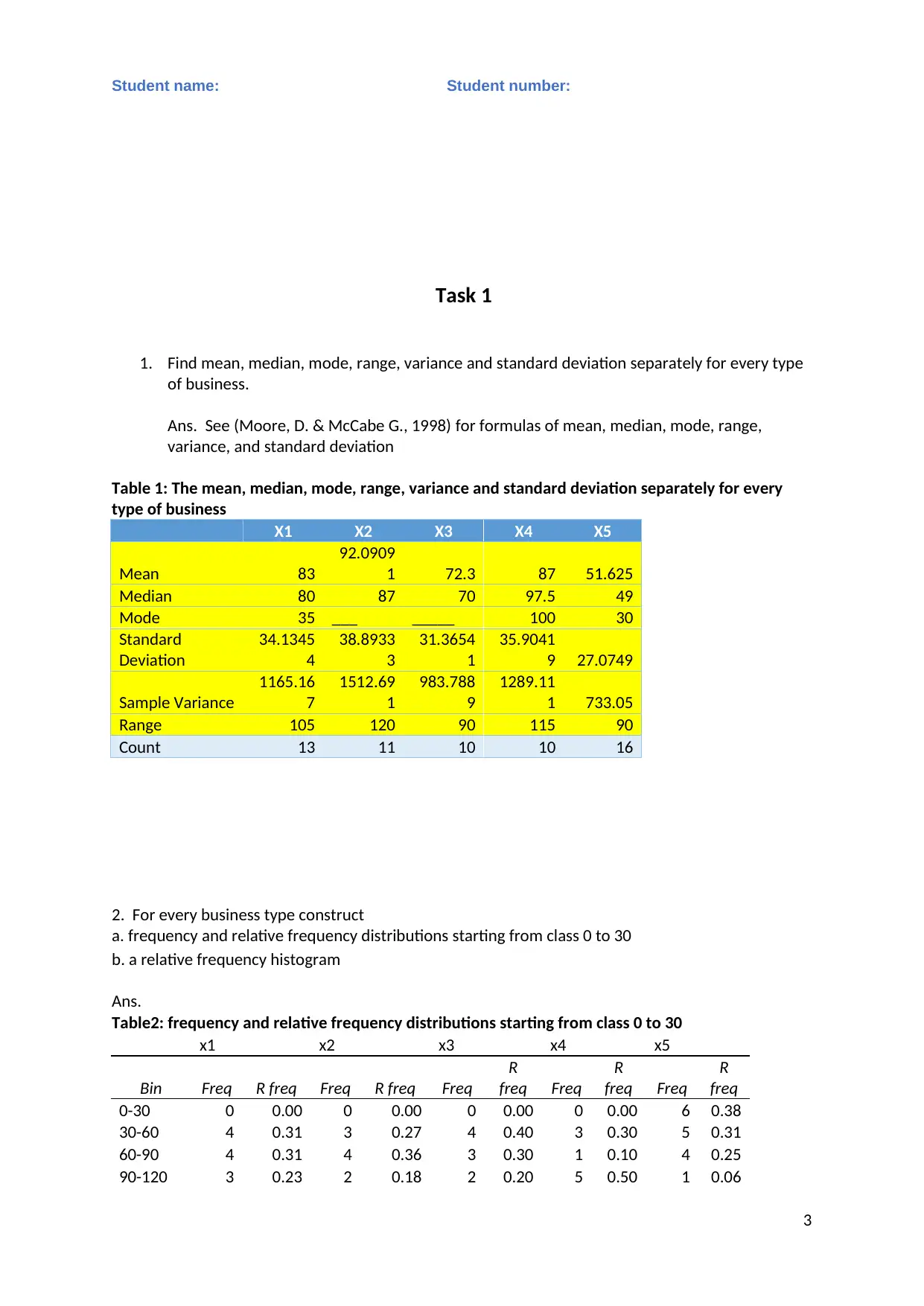
Ans. See (Moore, D. & McCabe G., 1998) for formulas of mean, median, mode, range,
variance, and standard deviation
Table 1: The mean, median, mode, range, variance and standard deviation separately for every
type of business
X1 X2 X3 X4 X5
Mean 83
92.0909
1 72.3 87 51.625
Median 80 87 70 97.5 49
Mode 35 ___ _____ 100 30
Standard
Deviation
34.1345
4
38.8933
3
31.3654
1
35.9041
9 27.0749
Sample Variance
1165.16
7
1512.69
1
983.788
9
1289.11
1 733.05
Range 105 120 90 115 90
Count 13 11 10 10 16
2. For every business type construct
a. frequency and relative frequency distributions starting from class 0 to 30
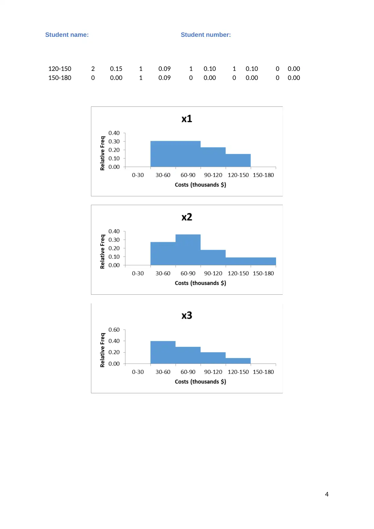
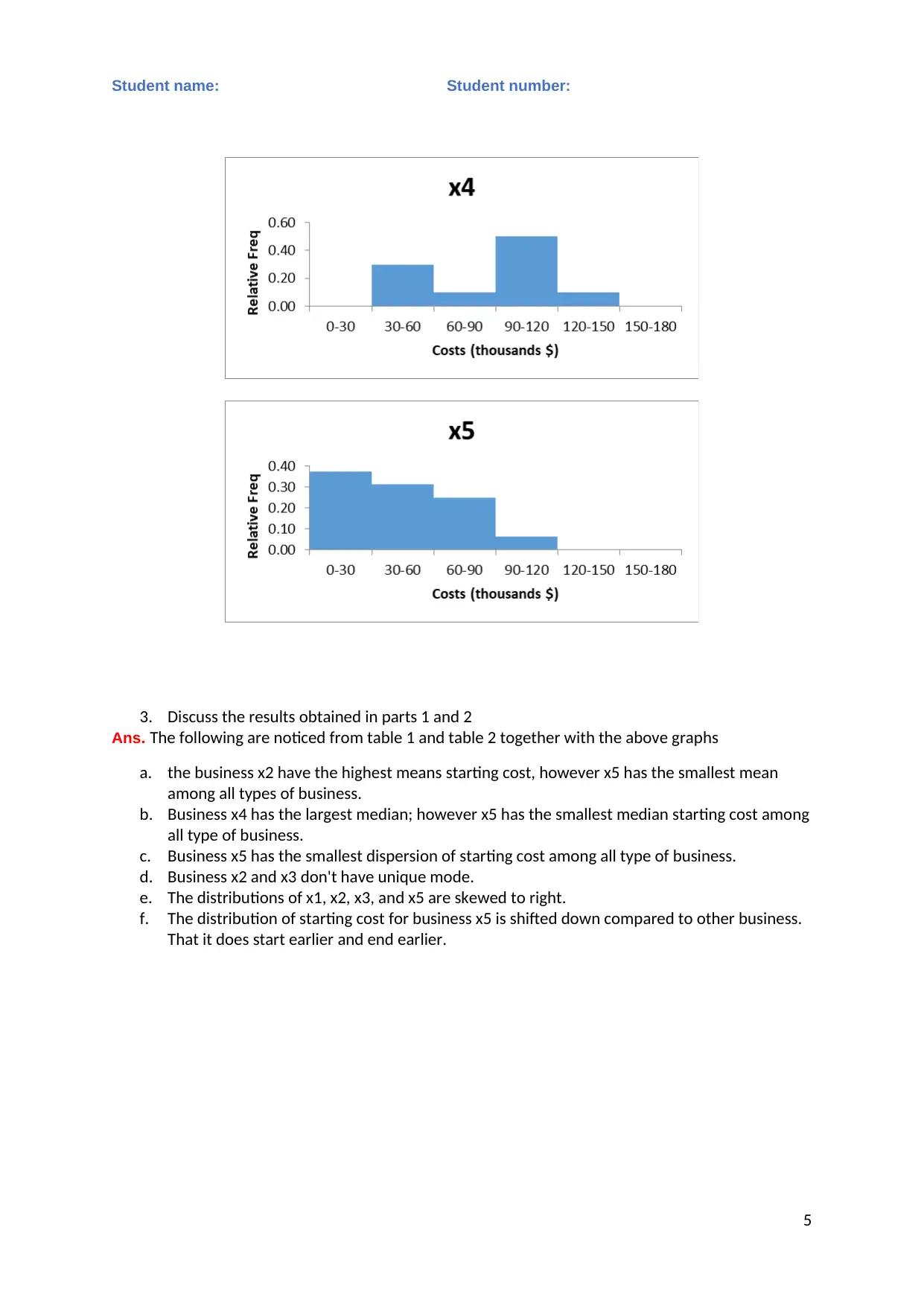
b. a relative frequency histogram
Ans.
Table2: frequency and relative frequency distributions starting from class 0 to 30
x1 x2 x3 x4 x5
Bin Freq R freq Freq R freq Freq
R
freq Freq
R
freq Freq
R
freq
0-30 0 0.00 0 0.00 0 0.00 0 0.00 6 0.38
30-60 4 0.31 3 0.27 4 0.40 3 0.30 5 0.31
60-90 4 0.31 4 0.36 3 0.30 1 0.10 4 0.25
90-120 3 0.23 2 0.18 2 0.20 5 0.50 1 0.06
3

Student name: Student number:
120-150 2 0.15 1 0.09 1 0.10 1 0.10 0 0.00
150-180 0 0.00 1 0.09 0 0.00 0 0.00 0 0.00
4

Student name: Student number:
3. Discuss the results obtained in parts 1 and 2
Ans. The following are noticed from table 1 and table 2 together with the above graphs
a. the business x2 have the highest means starting cost, however x5 has the smallest mean
among all types of business.
b. Business x4 has the largest median; however x5 has the smallest median starting cost among
all type of business.
c. Business x5 has the smallest dispersion of starting cost among all type of business.
d. Business x2 and x3 don't have unique mode.
e. The distributions of x1, x2, x3, and x5 are skewed to right.
f. The distribution of starting cost for business x5 is shifted down compared to other business.
That it does start earlier and end earlier.
5

Student name: Student number:
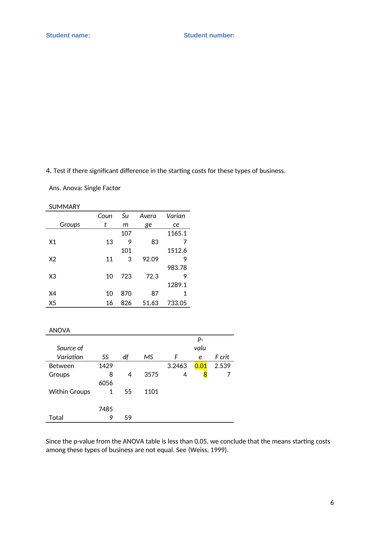
4. Test if there significant difference in the starting costs for these types of business.
Ans. Anova: Single Factor
SUMMARY
Groups
Coun
t
Su
m
Avera
ge
Varian
ce
X1 13
107
9 83
1165.1
7
X2 11
101
3 92.09
1512.6
9
X3 10 723 72.3
983.78
9
X4 10 870 87
1289.1
1
X5 16 826 51.63 733.05
ANOVA
Source of
Variation SS df MS F
P-
valu
e F crit
Between
Groups
1429
8 4 3575
3.2463
4
0.01
8
2.539
7
Within Groups
6056
1 55 1101
Total
7485
9 59
Since the p-value from the ANOVA table is less than 0.05, we conclude that the means starting costs
among these types of business are not equal. See (Weiss, 1999).
6

Student name: Student number:
Task 2
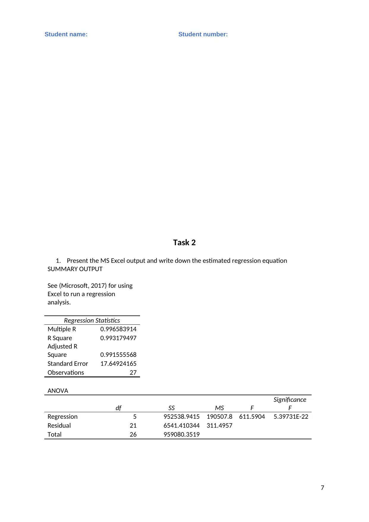
1. Present the MS Excel output and write down the estimated regression equation
SUMMARY OUTPUT
See (Microsoft, 2017) for using
Excel to run a regression
analysis.
Regression Statistics
Multiple R 0.996583914
R Square 0.993179497
Adjusted R
Square 0.991555568
Standard Error 17.64924165
Observations 27
ANOVA
df SS MS F
Significance
F
Regression 5 952538.9415 190507.8 611.5904 5.39731E-22
Residual 21 6541.410344 311.4957
Total 26 959080.3519
7

Student name: Student number:
Coefficients
Standard
Error t Stat P-value
Lower
95%
Upper
95%
Intercep
t -18.859 30.150 -0.626 0.538 -81.560 43.841
X2 16.202 3.544 4.571 0.000 8.831 23.573
X3 0.175 0.058 3.032 0.006 0.055 0.294
X4 11.526 2.532 4.552 0.000 6.260 16.792
X5 13.580 1.770 7.671 0.000 9.898 17.262
X6 -5.311 1.705 -3.114 0.005 -8.858 -1.764
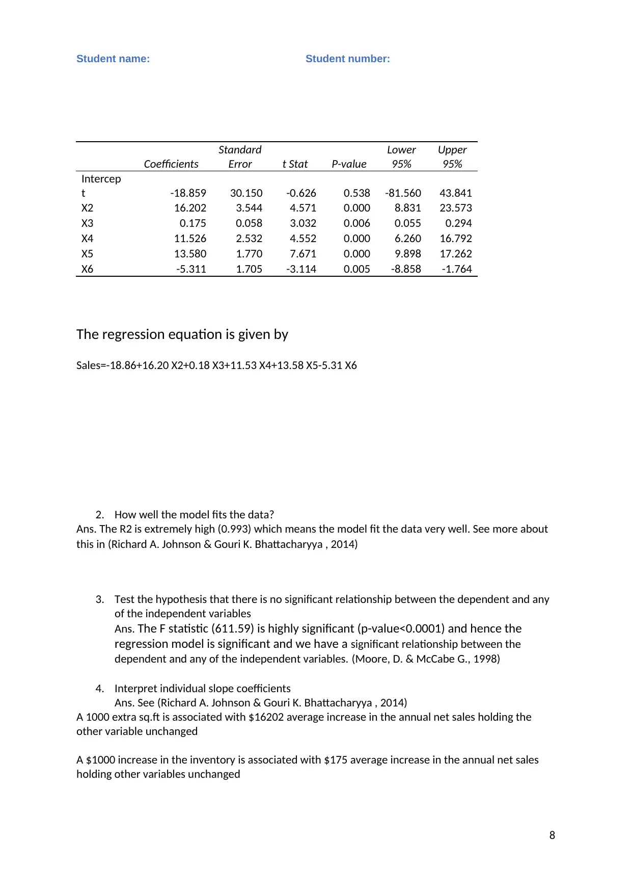
The regression equation is given by
Sales=-18.86+16.20 X2+0.18 X3+11.53 X4+13.58 X5-5.31 X6
2. How well the model fits the data?
Ans. The R2 is extremely high (0.993) which means the model fit the data very well. See more about
this in (Richard A. Johnson & Gouri K. Bhattacharyya , 2014)
3. Test the hypothesis that there is no significant relationship between the dependent and any
of the independent variables
Ans. The F statistic (611.59) is highly significant (p-value<0.0001) and hence the
regression model is significant and we have a significant relationship between the
dependent and any of the independent variables. (Moore, D. & McCabe G., 1998)
4. Interpret individual slope coefficients
Ans. See (Richard A. Johnson & Gouri K. Bhattacharyya , 2014)
A 1000 extra sq.ft is associated with $16202 average increase in the annual net sales holding the
other variable unchanged
A $1000 increase in the inventory is associated with $175 average increase in the annual net sales
holding other variables unchanged
8

Student name: Student number:
A $1000 increase in the amount spent on advertising is associated with $11526 increase in the
annual net sales holding other variables not changed
A 1000 extra sales district is associated by an average increase of $13580 in the annual net sales
holding other variables constants
A one more competitor store in the district is associated with an average decrease of $5311 in the
annual net salary holding other variables unchanged
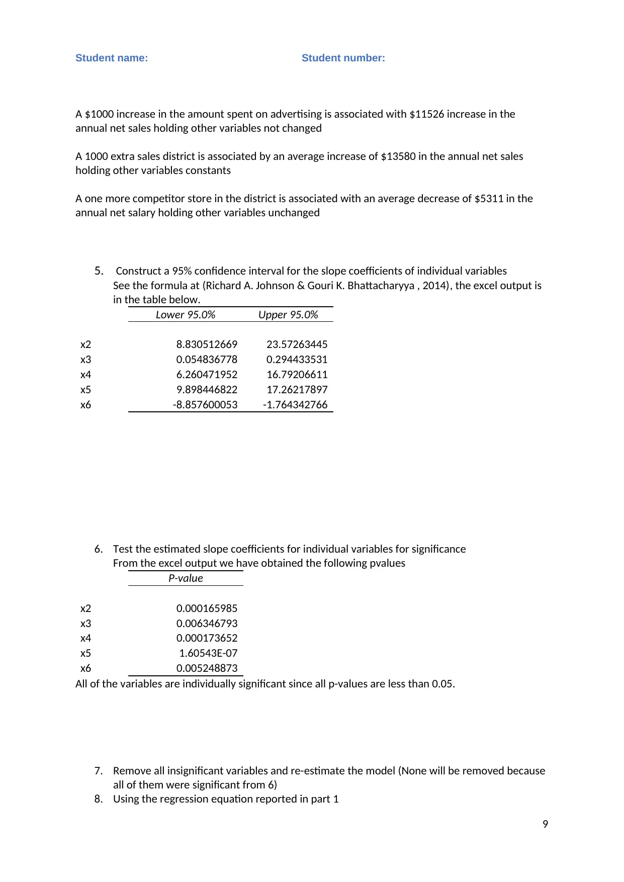
5. Construct a 95% confidence interval for the slope coefficients of individual variables
See the formula at (Richard A. Johnson & Gouri K. Bhattacharyya , 2014), the excel output is
in the table below.
Lower 95.0% Upper 95.0%
x2 8.830512669 23.57263445
x3 0.054836778 0.294433531
x4 6.260471952 16.79206611
x5 9.898446822 17.26217897
x6 -8.857600053 -1.764342766
6. Test the estimated slope coefficients for individual variables for significance
From the excel output we have obtained the following pvalues
P-value
x2 0.000165985
x3 0.006346793
x4 0.000173652
x5 1.60543E-07
x6 0.005248873
All of the variables are individually significant since all p-values are less than 0.05.
7. Remove all insignificant variables and re-estimate the model (None will be removed because
all of them were significant from 6)
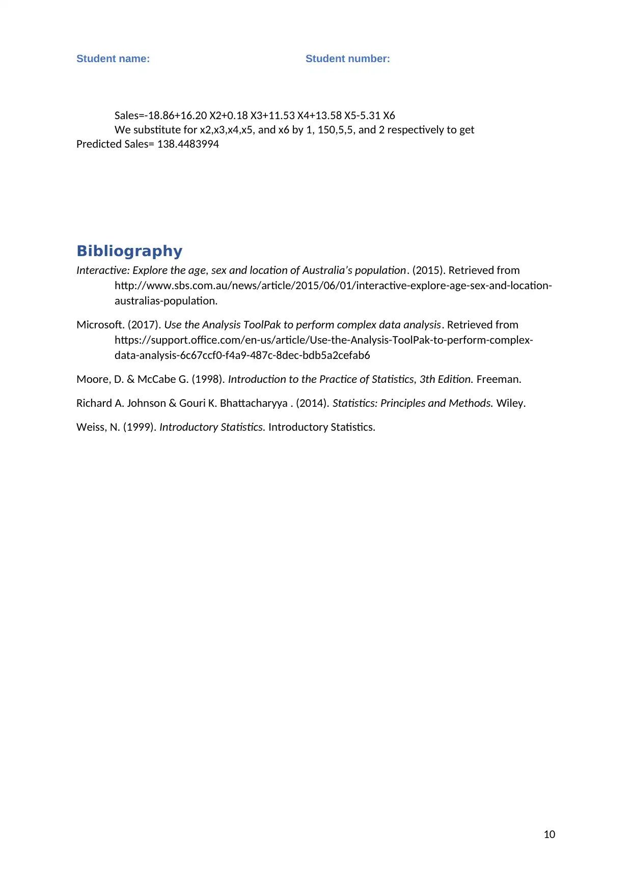
8. Using the regression equation reported in part 1
9

Student name: Student number:
Sales=-18.86+16.20 X2+0.18 X3+11.53 X4+13.58 X5-5.31 X6
We substitute for x2,x3,x4,x5, and x6 by 1, 150,5,5, and 2 respectively to get
Predicted Sales= 138.4483994
Bibliography
Interactive: Explore the age, sex and location of Australia’s population. (2015). Retrieved from
http://www.sbs.com.au/news/article/2015/06/01/interactive-explore-age-sex-and-location-
australias-population.
Microsoft. (2017). Use the Analysis ToolPak to perform complex data analysis. Retrieved from
https://support.office.com/en-us/article/Use-the-Analysis-ToolPak-to-perform-complex-
data-analysis-6c67ccf0-f4a9-487c-8dec-bdb5a2cefab6
Moore, D. & McCabe G. (1998). Introduction to the Practice of Statistics, 3th Edition. Freeman.
Richard A. Johnson & Gouri K. Bhattacharyya . (2014). Statistics: Principles and Methods. Wiley.
Weiss, N. (1999). Introductory Statistics. Introductory Statistics.
10