Statistical Analysis Assignment 2: Data Interpretation and Analysis

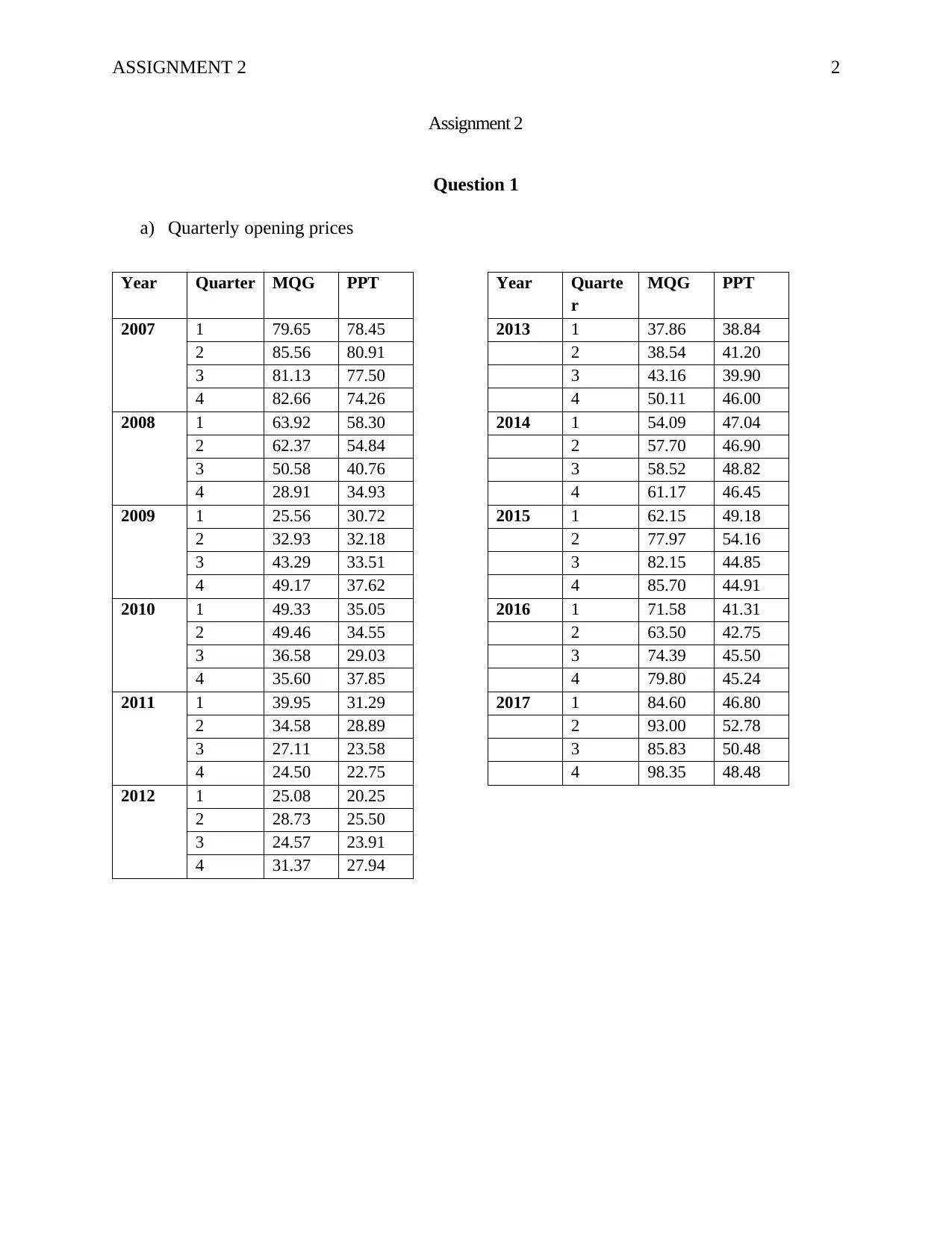
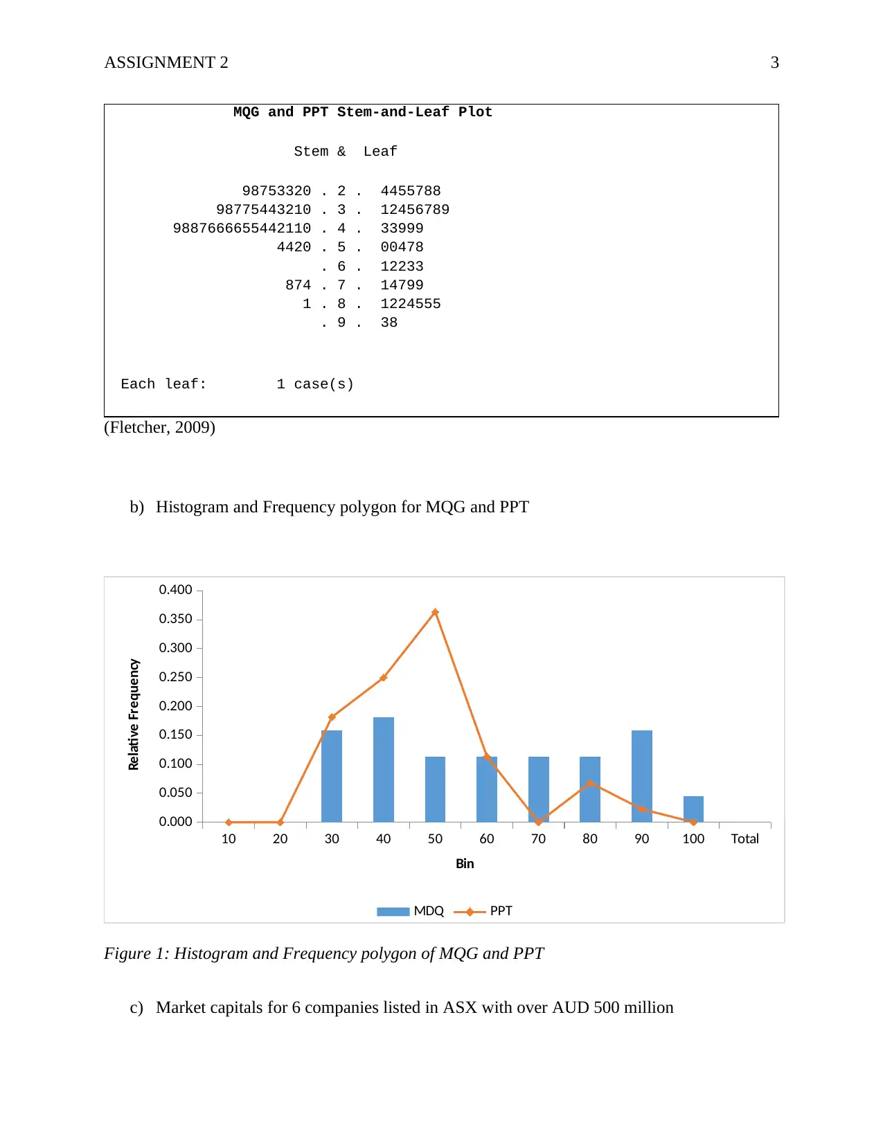
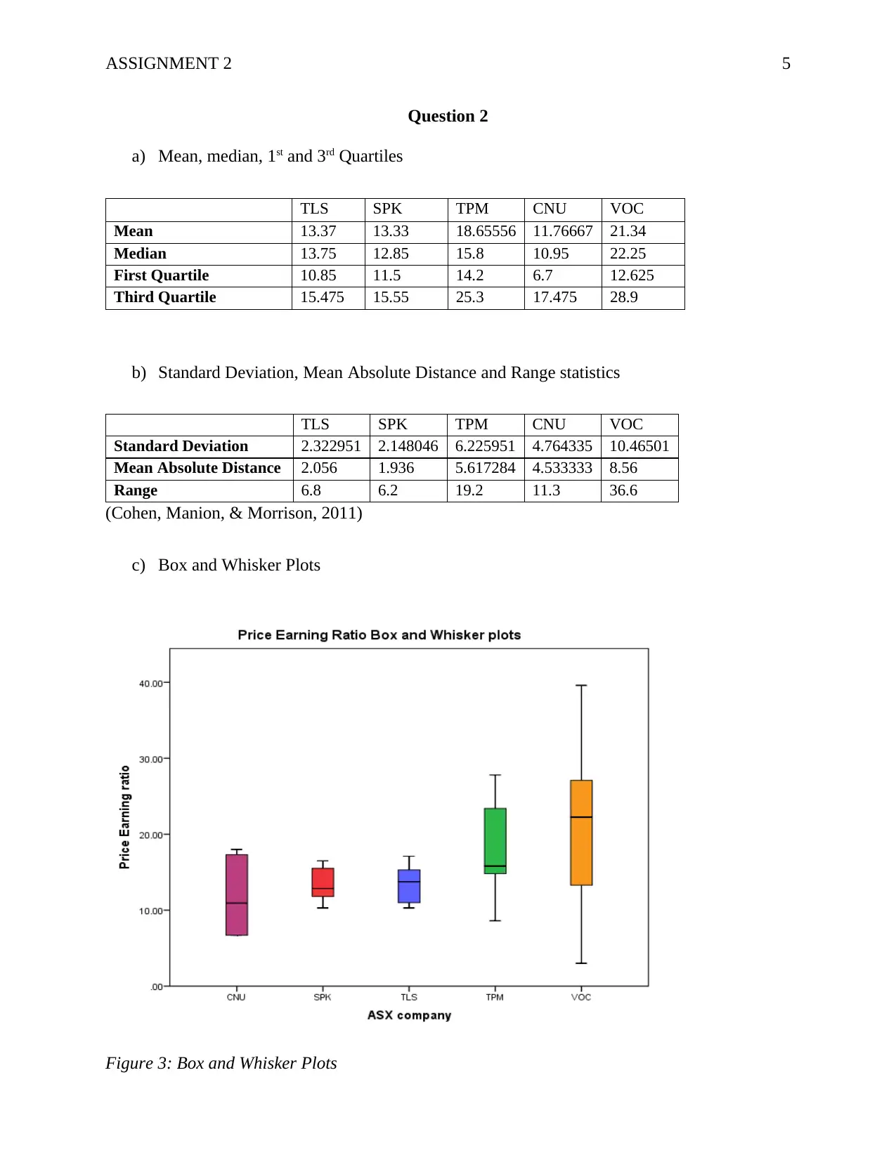
This assignment presents a comprehensive statistical analysis covering various topics. The first question involves analyzing quarterly opening stock prices for MQG and PPT, using stem-and-leaf plots, histograms, and frequency polygons to compare investment potential. The second question calculat...Read More

Running head: ASSIGNMENT 2
Assignment 2
Name
Course Number
Date
Faculty Name

ASSIGNMENT 2 2
Assignment 2
Question 1
a) Quarterly opening prices
Year Quarter MQG PPT Year Quarte
r
MQG PPT
2007 1 79.65 78.45 2013 1 37.86 38.84
2 85.56 80.91 2 38.54 41.20
3 81.13 77.50 3 43.16 39.90
4 82.66 74.26 4 50.11 46.00
2008 1 63.92 58.30 2014 1 54.09 47.04
2 62.37 54.84 2 57.70 46.90
3 50.58 40.76 3 58.52 48.82
4 28.91 34.93 4 61.17 46.45
2009 1 25.56 30.72 2015 1 62.15 49.18
2 32.93 32.18 2 77.97 54.16
3 43.29 33.51 3 82.15 44.85
4 49.17 37.62 4 85.70 44.91
2010 1 49.33 35.05 2016 1 71.58 41.31
2 49.46 34.55 2 63.50 42.75
3 36.58 29.03 3 74.39 45.50
4 35.60 37.85 4 79.80 45.24
2011 1 39.95 31.29 2017 1 84.60 46.80
2 34.58 28.89 2 93.00 52.78
3 27.11 23.58 3 85.83 50.48
4 24.50 22.75 4 98.35 48.48
2012 1 25.08 20.25
2 28.73 25.50
3 24.57 23.91
4 31.37 27.94

ASSIGNMENT 2 3
MQG and PPT Stem-and-Leaf Plot
Stem & Leaf
98753320 . 2 . 4455788
98775443210 . 3 . 12456789
9887666655442110 . 4 . 33999
4420 . 5 . 00478
. 6 . 12233
874 . 7 . 14799
1 . 8 . 1224555
. 9 . 38
Each leaf: 1 case(s)
(Fletcher, 2009)
b) Histogram and Frequency polygon for MQG and PPT
10 20 30 40 50 60 70 80 90 100 Total
0.000
0.050
0.100
0.150
0.200
0.250
0.300
0.350
0.400
MDQ PPT
Bin
Relative Frequency
Figure 1: Histogram and Frequency polygon of MQG and PPT
c) Market capitals for 6 companies listed in ASX with over AUD 500 million

ASSIGNMENT 2 4
Perpetual Limited
Macquarie Group Limited
APA GROUP
Aristocrat Leisure
Ramsay Health Care
Stockland Units/ Stapled Securities
AUD
1,869,000,000.00
AUD
37,072,000,000.00
AUD
9,690,000,000.00
AUD
17,125,800,000.00
AUD
13,072,600,000.00
AUD
10,078,700,000.00
Market Capitals
Figure 2: Market capitals
d) Invest in MQG or PPT
Based on the series of previous share prices from 2007 to March 2018, I would advise on
investing with PPT because the prices are down and there is a possibility of a rise in a few
moments. This is in comparison to MQG whose prices have been rising since 2010 and just as
any other stock price, there are very high chance of the prices losing value. Therefore, it would
be more advisable to invest in a stock whose price has a higher chance of increasing than
decreasing. In addition, PPT has a higher dividend yield of 6.65% compared to MQG which is
4.66%. Further, PPT has a lower Price-earning Ration compared to MQG, which make PPT
stock better to invest in because their future growth has higher chances of growth(Aspara, 2009;
Lynott, 2005).

ASSIGNMENT 2 5
Question 2
a) Mean, median, 1st and 3rd Quartiles
TLS SPK TPM CNU VOC
Mean 13.37 13.33 18.65556 11.76667 21.34
Median 13.75 12.85 15.8 10.95 22.25
First Quartile 10.85 11.5 14.2 6.7 12.625
Third Quartile 15.475 15.55 25.3 17.475 28.9
b) Standard Deviation, Mean Absolute Distance and Range statistics
TLS SPK TPM CNU VOC
Standard Deviation 2.322951 2.148046 6.225951 4.764335 10.46501
Mean Absolute Distance 2.056 1.936 5.617284 4.533333 8.56
Range 6.8 6.2 19.2 11.3 36.6
(Cohen, Manion, & Morrison, 2011)
c) Box and Whisker Plots
Figure 3: Box and Whisker Plots

ASSIGNMENT 2 6
d) A discussion on the price-earnings ratio values
Higher values of price-earnings ratio show that the stock is overpriced while stocks with small
values are seen to be better because they have higher growth potentials. Therefore, CNU has the
highest growth potential compared to the others because the median measure small compared to
the others. However, SPK has the least margin for the 3rd and 1st quartile, hence lower deviation
from the median. It is very risky to invest in VOC stock because it is hard to estimate its ideal
price-earnings ratio because of the higher variation. Therefore, it will be safer to invest in CNU,
SPK and TLS stock as opposed to TPM and VOC(Titman, Wei, & Xie, 2004).
Question 3
a) The probability that an Australian will die from neoplasms.
44674
147678 =0.3025
b) The probability of a Female Australian to die from disease of the circulatory system
22493
71896 =0.313
c) Proportions of deaths
The disease with the highest proportion of male deaths compared to female deaths is Neoplasms
with a difference of 6.3%. Diseases of circulatory system such as heart disease have the highest
difference in proportion between female deaths and male deaths with a difference of 3.4%.
d) The probability of dying from diabetes mellitus
male= 2298
75782=0.0303

ASSIGNMENT 2 7
female= 2030
71896 =0.0282
overrall = 4328
147678 =0.0293
(McCluskey & Lalkhen, 2007)
Question 4
a) Probability of rainfall
i. The probability that there will be no rainfall in any given day
yearly rate of rainfall (λ yr)= number of days withrainfall
365 =230
365 =0.63
Weekly rate of rainfall( λwk )= 0.63
52 =0.0121
daily rate( λday )= 0.012118
7 =0.00173
P ( 0 )= λwk
0
0 ! ∗e− λwk
=e−λwk
=e−0.0121=0.988
ii. The probability of 2 or more days of rainfall in a week
P ( 2∨more days of rainfall )=1−P ( 0 ) −P ( 1 )
P ( 0 )= λday
0
0 ! ∗e− λday
=e−0.0017=0.998

ASSIGNMENT 2 8
P ( 1 )= 0.0017
1 ∗0.998=0.0017
P ( 2∨more days of rainfall∈a week ) =1−0.998−0.0017=0.0003
b) Assuming that the weekly rainfall follows a normal distribution
The mean weekly rainfall is 9.9132mm and a standard deviation of 12.297mm
i) The probability of having rainfall between 5mm to 15mm
5−9.9132
12.297 >Z> 15−9.9132
12.297
−0.4 >Z >0.414
0.6591−0.3446=0.3145
ii) Amount of rainfall if only 10% of the weeks have that amount of rainfall or higher
1.28= X −9.9132
12.297
X = ( 1.28∗12.297 ) + 9.9132 (Tsokos, Wooten, Tsokos, & Wooten, 2016)
The amount of rainfall will be 25.653 mm
Question 5
a) Normality Test
Refractive Index

ASSIGNMENT 2 9
Figure 4: Refractive index for refractive index
Sodium
Figure 5: Probability plot for Sodium
Magnesium

ASSIGNMENT 2 10
Figure 6: Probability plot of Magnesium
Aluminium
Figure 7: Probability plot of Aluminium
Silicon

ASSIGNMENT 2 11
Figure 8: Probability plot of Silicon
Potassium
Figure 9: Probability plot of Potassium
Calcium

ASSIGNMENT 2 12
Figure 10: Probability plot of Calcium
Barium
Figure 11: Probability plot of Barium
Iron

ASSIGNMENT 2 13
Figure 12: Probability plot of iron
Refractive index, Silicon, Aluminium, and Sodium are the only variables which are
approximately normally distributed(Abdal-sahib et al., 2013; Tsokos et al., 2016).
b) Confidence intervals of Float and non-float glass
Float Glass
Table 1: Float Glass Confidence intervals for normally distributed variables
Statistic Std. Error
Refractive index Mean 1.5185708 .00023735
95% Confidence Interval for
Mean
Lower Bound 1.5180990
Upper Bound 1.5190426
Sodium Mean 13.2803 .05402
95% Confidence Interval for
Mean
Lower Bound 13.1730
Upper Bound 13.3877
Aluminum Mean 1.1711 .03080
95% Confidence Interval for
Mean
Lower Bound 1.1099
Upper Bound 1.2324
Silicon Mean 72.5772 .06030
95% Confidence Interval for
Mean
Lower Bound 72.4574
Upper Bound 72.6971

ASSIGNMENT 2 14
Non-Float Glass
Table 2: Non-Float Glass Confidence intervals for normally distributed variables
Statistic Std. Error
Refractive index Mean 1.5186186 .00043613
95% Confidence Interval for
Mean
Lower Bound 1.5177497
Upper Bound 1.5194874
Sodium Mean 13.1117 .07618
95% Confidence Interval for
Mean
Lower Bound 12.9599
Upper Bound 13.2635
Aluminum Mean 1.4082 .03652
95% Confidence Interval for
Mean
Lower Bound 1.3354
Upper Bound 1.4809
Silicon Mean 72.5980 .08311
95% Confidence Interval for
Mean
Lower Bound 72.4325
Upper Bound 72.7636

ASSIGNMENT 2 15
References
Abdal-sahib, R., Altammar, S. M., Azlan, H. A., Aytemur, A., Balters, S., Steinert, M., …
Canny, J. (2013). Testing for Normality. Frontiers in Psychology, 98(1), 1–8.
https://doi.org/10.3389/fpsyg.2014.01470
Aspara, J. (2009). Aesthetics of stock investments. Consumption Markets & Culture, 12(2), 99–
131. https://doi.org/10.1080/10253860902840917
Cohen, L., Manion, L., & Morrison, K. (2011). Descriptive Statistics. In Research methods in
education (pp. 622–640). https://doi.org/10.1213/ANE.0000000000002471
Fletcher, J. (2009). Normal distribution. BMJ, 338(feb18 2), b646–b646.
https://doi.org/10.1136/bmj.b646
Lynott, W. J. (2005). Stock investments. Water Well Journal, 59(12), 39. Retrieved from
http://www.scopus.com/inward/record.url?eid=2-s2.0-
30344484585&partnerID=40&md5=ba73235c348c82cf518a1f10cd84cbe4
McCluskey, A., & Lalkhen, A. G. (2007). Statistics III: Probability and statistical tests.s, 7(5),
167–170. https://doi.org/10.1093/bjaceaccp/mkm028
Titman, S., Wei, K. C. J., & Xie, F. (2004). Capital Investments and Stock Returns. Journal of
Financial and Quantitative Analysis, 39(04), 677.
https://doi.org/10.1017/S0022109000003173
Tsokos, C., Wooten, R., Tsokos, C., & Wooten, R. (2016). Normal Probability. In The Joy of
Finite Mathematics (pp. 231–263). https://doi.org/10.1016/B978-0-12-802967-1.00007-3