Business Intelligence Report: House Price Prediction using Data Mining
VerifiedAdded on 2023/06/12
|12
|2112
|315
Report
AI Summary
This report demonstrates the application of data mining techniques for business intelligence, focusing on house price prediction. It begins with Exploratory Data Analysis (EDA) using RapidMiner to understand data distribution and identify relevant variables. Correlation analysis and Chi-square tests are then employed to refine variable selection. Linear regression is used to model the impact of key variables (sqft_living, grade, sqft_living15, sqft_above, and bathrooms) on house prices, resulting in a predictive equation. Finally, Tableau is used to visualize house prices from 2014-2015, including a text table summarizing key metrics by quarter and a geographic map illustrating price variations across different locations. Desklib provides access to this and other solved assignments for students.
Running head: IT
IT
Name of the Student:
Name of the University:
Author’s Note:
IT
Name of the Student:
Name of the University:
Author’s Note:
Paraphrase This Document
Need a fresh take? Get an instant paraphrase of this document with our AI Paraphraser
1IT
Table of Contents
1A: EDA and Linear Regression Analysis.................................................................................3
1.1 EDA..................................................................................................................................3
1.2 Correlation........................................................................................................................4
1.3 Chi-Square........................................................................................................................5
1B: Linear Regression Analysis.................................................................................................6
2: Tableau Representation of House Prices (2014-2015)..........................................................8
2.1 Text Table or Graph view................................................................................................8
2.2 GeoMap............................................................................................................................9
References................................................................................................................................11
2IT
The purpose of the present assignment is an attempt to gain business intelligence
through the application of applied knowledge of the people in finances, markets, management
and technology. In order to gain business intelligence one needs to apply data mining process.
The mined data can be visually represented as a graph or chart. For this assignment we would
use RapidMiner for data mining and Tableau for data visualization (Witten 2016).
In the first part of the report Rapidminer software is used to get an insight into the
house prices data. Initially the data is explored to understand how the information in the data
is distributed. This is followed by doing correlation analysis wherein variables which are
closely related with house prices are chosen. This is further enhanced with the help of Chi-
square test. Finally, regression analysis is used to unravel how selected variables impact the
prices of the houses.
⊘ This is a preview!⊘
Do you want full access?
Subscribe today to unlock all pages.
Trusted by 1+ million students worldwide
3IT
1A: EDA and Linear Regression Analysis
The analysis of the present data is incorporated in two stage process. In the first stage the data
is analysed with use of “Rapidminer”. In the next stage, important information about the data
is visualised with the help of “Tableau”. For the primary stage prior to form an equation to
represent the house prices, the data is explored and variables are selected by process of
rejection. Finally, we construct an equation that can be used to represent the house prices
(Wu and Brynjolfsson 2015).
1.1 EDA
Paraphrase This Document
Need a fresh take? Get an instant paraphrase of this document with our AI Paraphraser
4IT
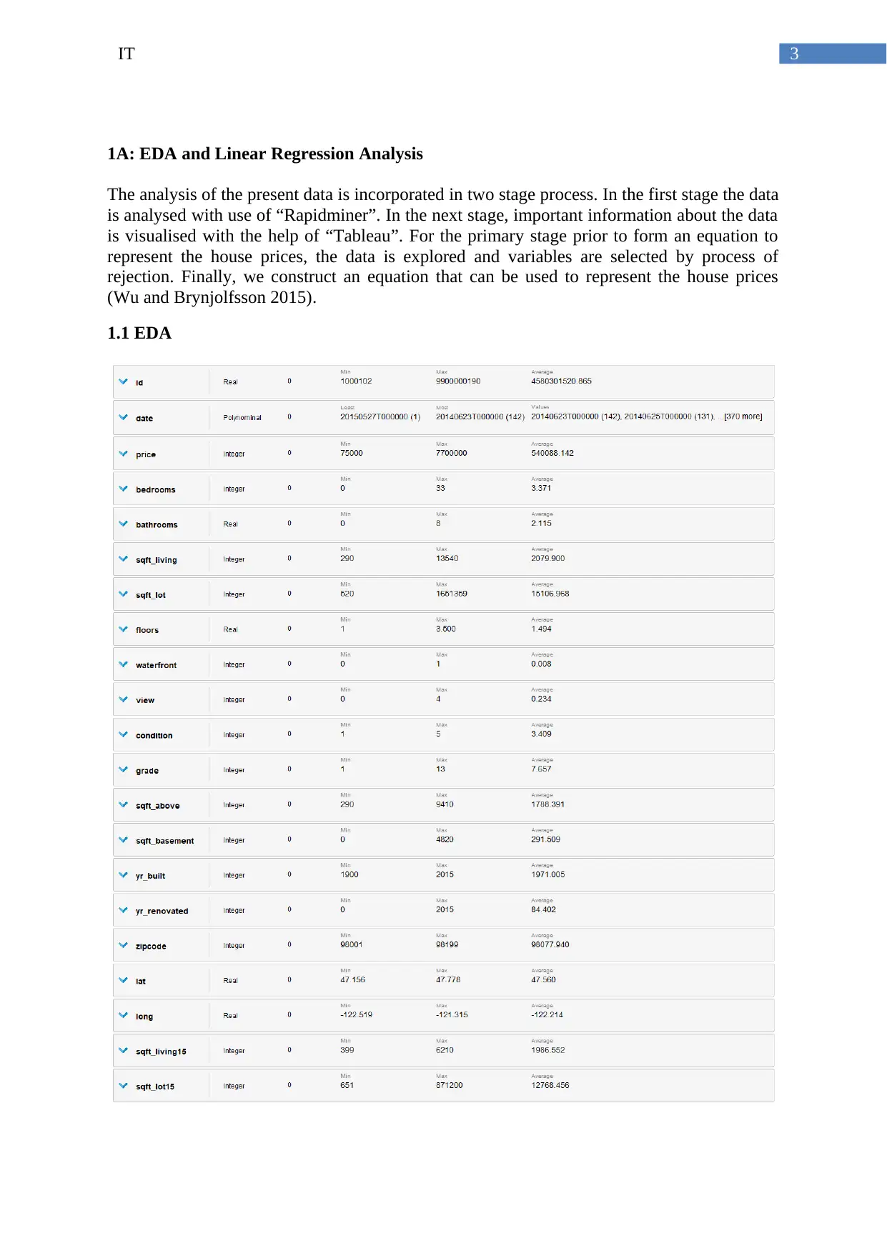
The purpose of primary process to gain information regarding a dataset is to conduct a
summary statistic. In “Rapidminer” software, exploratory data analysis (EDA) provides some
basic information about the data. In “Rapidminer”, the data of house prices is linked with
EDA. The information from the EDA suggested that the most of the variables were integers.
However, some of the variables were real also. The minimum, maximum and average value
of most of the variables were acquired (Larose and Larose 2014).
1.2 Correlation
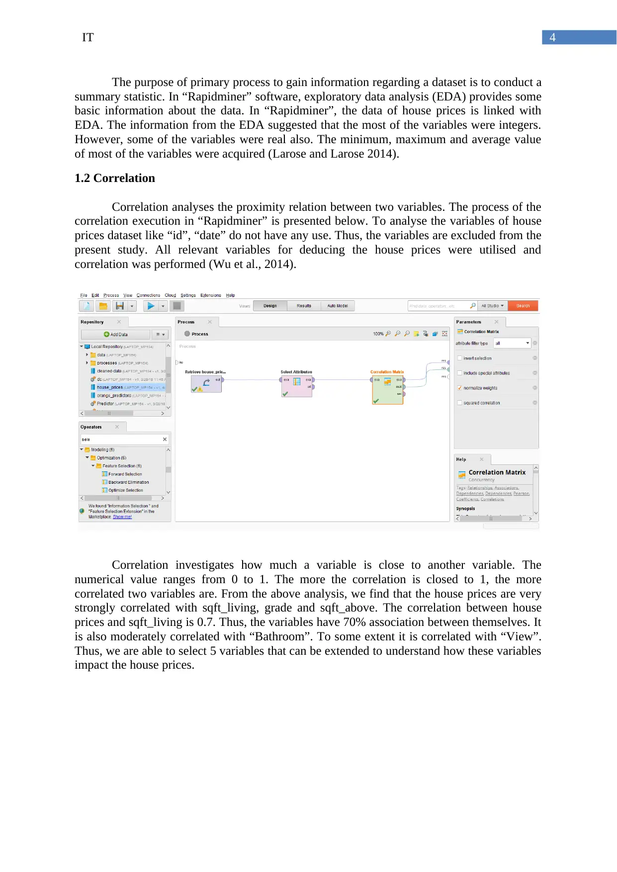
Correlation analyses the proximity relation between two variables. The process of the
correlation execution in “Rapidminer” is presented below. To analyse the variables of house
prices dataset like “id”, “date” do not have any use. Thus, the variables are excluded from the
present study. All relevant variables for deducing the house prices were utilised and
correlation was performed (Wu et al., 2014).
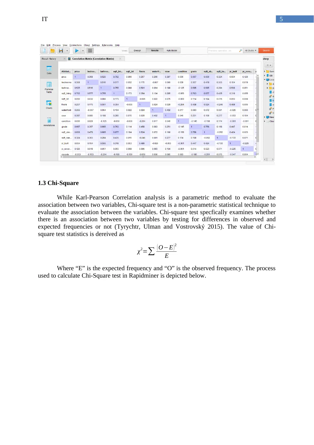
Correlation investigates how much a variable is close to another variable. The
numerical value ranges from 0 to 1. The more the correlation is closed to 1, the more
correlated two variables are. From the above analysis, we find that the house prices are very
strongly correlated with sqft_living, grade and sqft_above. The correlation between house
prices and sqft_living is 0.7. Thus, the variables have 70% association between themselves. It
is also moderately correlated with “Bathroom”. To some extent it is correlated with “View”.
Thus, we are able to select 5 variables that can be extended to understand how these variables
impact the house prices.
The purpose of primary process to gain information regarding a dataset is to conduct a
summary statistic. In “Rapidminer” software, exploratory data analysis (EDA) provides some
basic information about the data. In “Rapidminer”, the data of house prices is linked with
EDA. The information from the EDA suggested that the most of the variables were integers.
However, some of the variables were real also. The minimum, maximum and average value
of most of the variables were acquired (Larose and Larose 2014).
1.2 Correlation
Correlation analyses the proximity relation between two variables. The process of the
correlation execution in “Rapidminer” is presented below. To analyse the variables of house
prices dataset like “id”, “date” do not have any use. Thus, the variables are excluded from the
present study. All relevant variables for deducing the house prices were utilised and
correlation was performed (Wu et al., 2014).
Correlation investigates how much a variable is close to another variable. The
numerical value ranges from 0 to 1. The more the correlation is closed to 1, the more
correlated two variables are. From the above analysis, we find that the house prices are very
strongly correlated with sqft_living, grade and sqft_above. The correlation between house
prices and sqft_living is 0.7. Thus, the variables have 70% association between themselves. It
is also moderately correlated with “Bathroom”. To some extent it is correlated with “View”.
Thus, we are able to select 5 variables that can be extended to understand how these variables
impact the house prices.
5IT
1.3 Chi-Square
While Karl-Pearson Correlation analysis is a parametric method to evaluate the
association between two variables, Chi-square test is a non-parametric statistical technique to
evaluate the association between the variables. Chi-square test specfically examines whether
there is an association between two variables by testing for differences in observed and
expected frequencies or not (Tyrychtr, Ulman and Vostrovský 2015). The value of Chi-
square test statistics is dereived as
χ2=∑ ( O−E )2
E
Where “E” is the expected frequency and “O” is the observed frequency. The process
used to calculate Chi-Square test in Rapidminer is depicted below.
⊘ This is a preview!⊘
Do you want full access?
Subscribe today to unlock all pages.
Trusted by 1+ million students worldwide
6IT
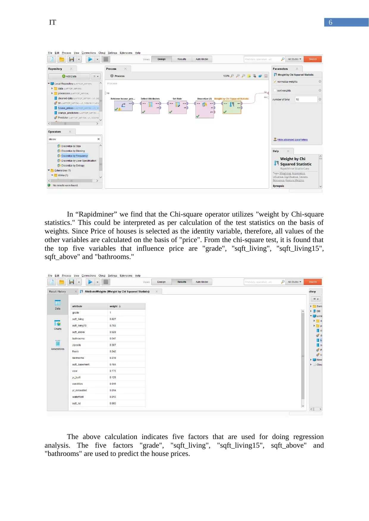
In “Rapidminer” we find that the Chi-square operator utilizes "weight by Chi-square
statistics." This could be interpreted as per calculation of the test statistics on the basis of
weights. Since Price of houses is selected as the identity variable, therefore, all values of the
other variables are calculated on the basis of "price". From the chi-square test, it is found that
the top five variables that influence price are "grade", "sqft_living", "sqft_living15",
sqft_above" and "bathrooms."
The above calculation indicates five factors that are used for doing regression
analysis. The five factors "grade", "sqft_living", "sqft_living15", sqft_above" and
"bathrooms" are used to predict the house prices.
Paraphrase This Document
Need a fresh take? Get an instant paraphrase of this document with our AI Paraphraser
7IT
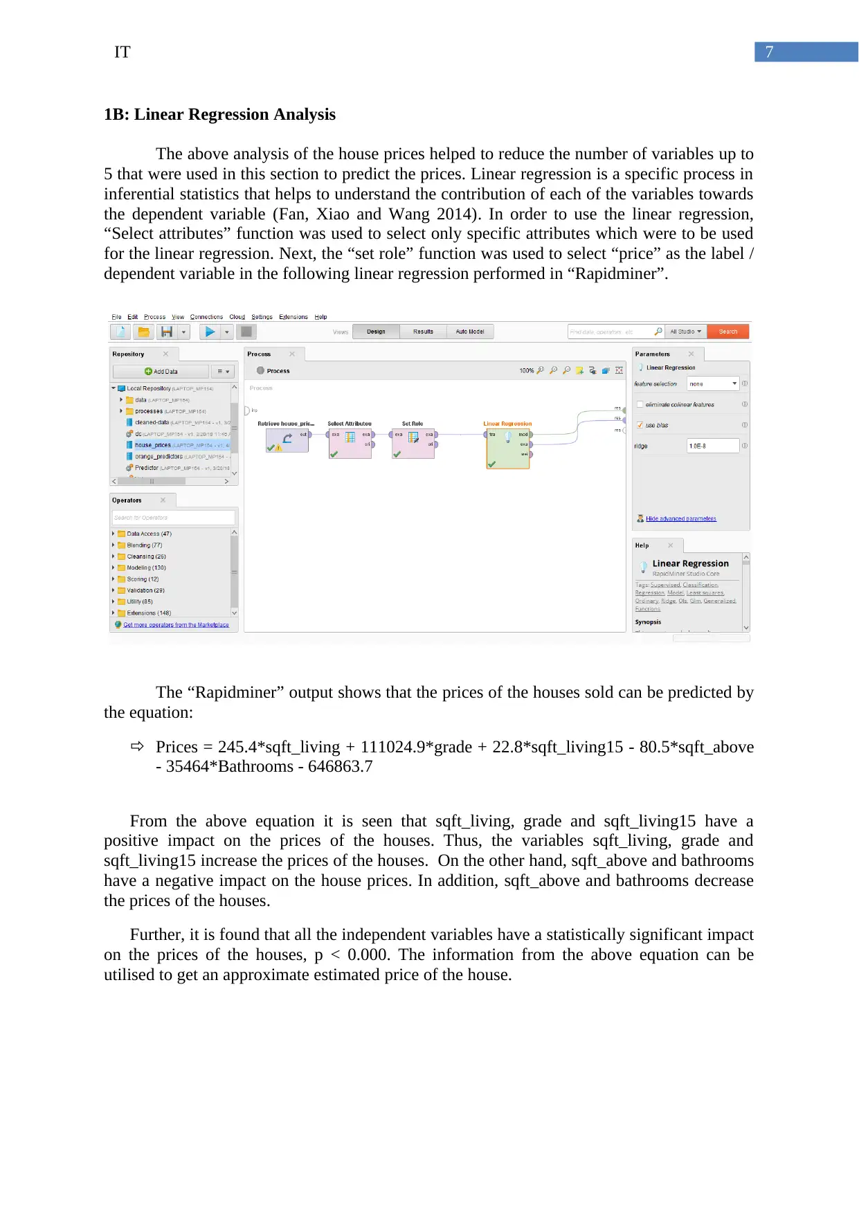
1B: Linear Regression Analysis
The above analysis of the house prices helped to reduce the number of variables up to
5 that were used in this section to predict the prices. Linear regression is a specific process in
inferential statistics that helps to understand the contribution of each of the variables towards
the dependent variable (Fan, Xiao and Wang 2014). In order to use the linear regression,
“Select attributes” function was used to select only specific attributes which were to be used
for the linear regression. Next, the “set role” function was used to select “price” as the label /
dependent variable in the following linear regression performed in “Rapidminer”.
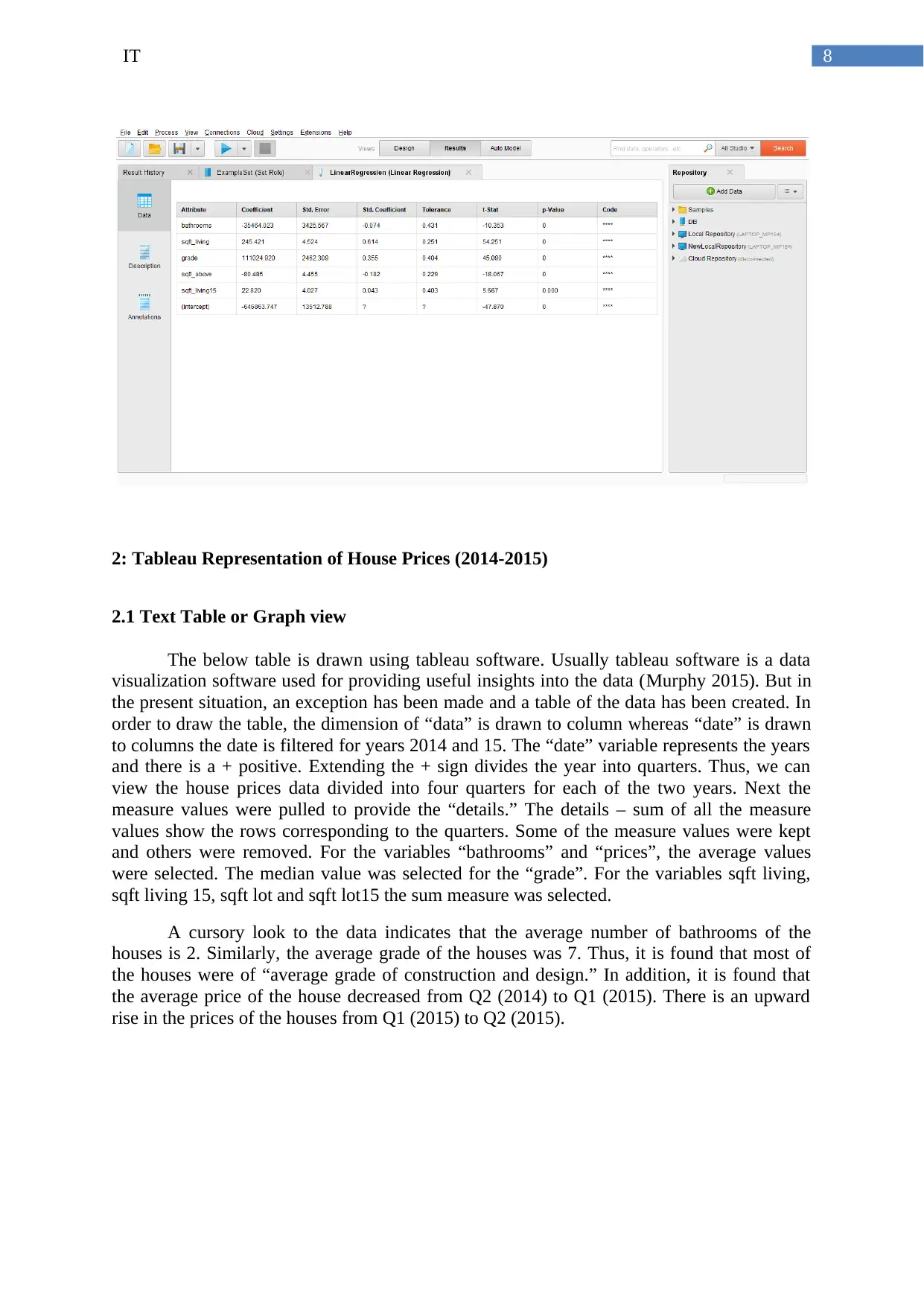
The “Rapidminer” output shows that the prices of the houses sold can be predicted by
the equation:
Prices = 245.4*sqft_living + 111024.9*grade + 22.8*sqft_living15 - 80.5*sqft_above
- 35464*Bathrooms - 646863.7
From the above equation it is seen that sqft_living, grade and sqft_living15 have a
positive impact on the prices of the houses. Thus, the variables sqft_living, grade and
sqft_living15 increase the prices of the houses. On the other hand, sqft_above and bathrooms
have a negative impact on the house prices. In addition, sqft_above and bathrooms decrease
the prices of the houses.
Further, it is found that all the independent variables have a statistically significant impact
on the prices of the houses, p < 0.000. The information from the above equation can be
utilised to get an approximate estimated price of the house.
1B: Linear Regression Analysis
The above analysis of the house prices helped to reduce the number of variables up to
5 that were used in this section to predict the prices. Linear regression is a specific process in
inferential statistics that helps to understand the contribution of each of the variables towards
the dependent variable (Fan, Xiao and Wang 2014). In order to use the linear regression,
“Select attributes” function was used to select only specific attributes which were to be used
for the linear regression. Next, the “set role” function was used to select “price” as the label /
dependent variable in the following linear regression performed in “Rapidminer”.
The “Rapidminer” output shows that the prices of the houses sold can be predicted by
the equation:
Prices = 245.4*sqft_living + 111024.9*grade + 22.8*sqft_living15 - 80.5*sqft_above
- 35464*Bathrooms - 646863.7
From the above equation it is seen that sqft_living, grade and sqft_living15 have a
positive impact on the prices of the houses. Thus, the variables sqft_living, grade and
sqft_living15 increase the prices of the houses. On the other hand, sqft_above and bathrooms
have a negative impact on the house prices. In addition, sqft_above and bathrooms decrease
the prices of the houses.
Further, it is found that all the independent variables have a statistically significant impact
on the prices of the houses, p < 0.000. The information from the above equation can be
utilised to get an approximate estimated price of the house.
8IT
2: Tableau Representation of House Prices (2014-2015)
2.1 Text Table or Graph view
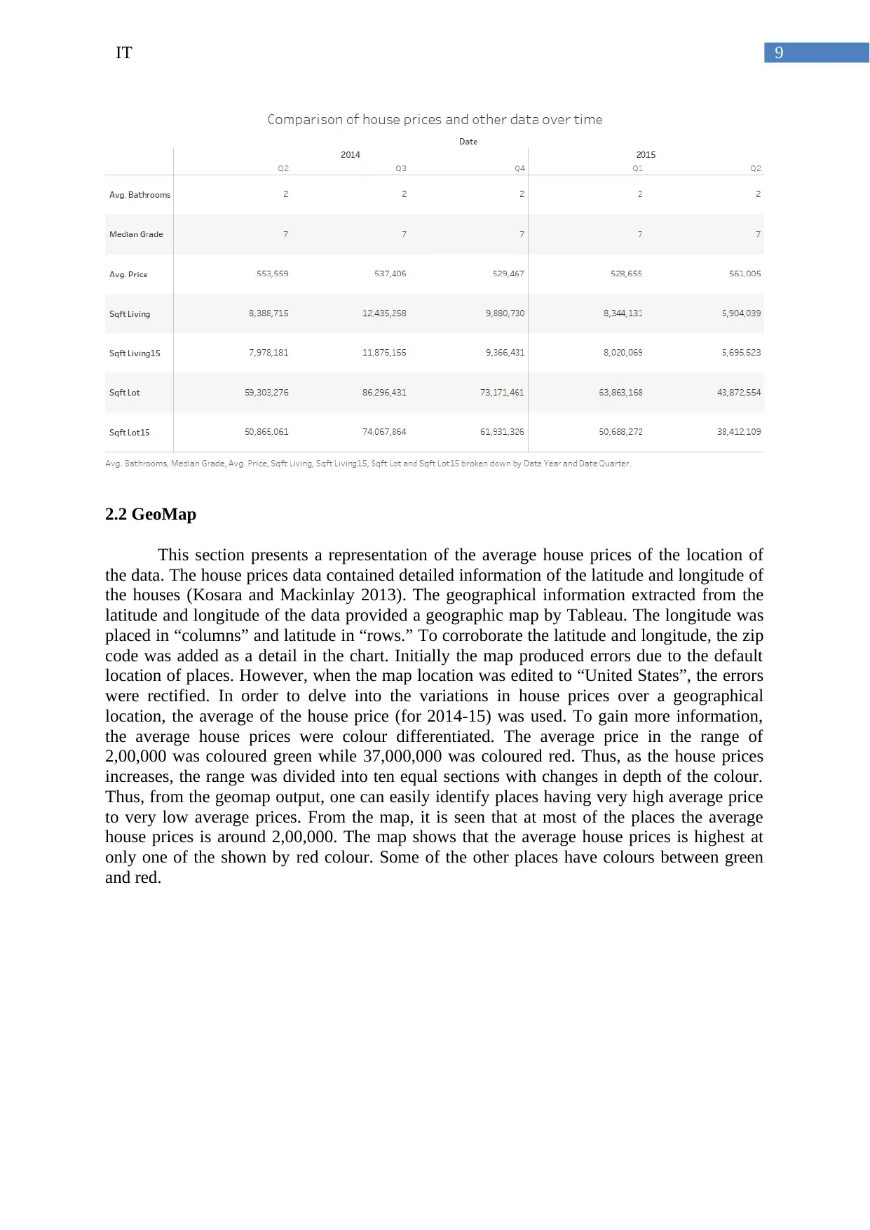
The below table is drawn using tableau software. Usually tableau software is a data
visualization software used for providing useful insights into the data (Murphy 2015). But in
the present situation, an exception has been made and a table of the data has been created. In
order to draw the table, the dimension of “data” is drawn to column whereas “date” is drawn
to columns the date is filtered for years 2014 and 15. The “date” variable represents the years
and there is a + positive. Extending the + sign divides the year into quarters. Thus, we can
view the house prices data divided into four quarters for each of the two years. Next the
measure values were pulled to provide the “details.” The details – sum of all the measure
values show the rows corresponding to the quarters. Some of the measure values were kept
and others were removed. For the variables “bathrooms” and “prices”, the average values
were selected. The median value was selected for the “grade”. For the variables sqft living,
sqft living 15, sqft lot and sqft lot15 the sum measure was selected.
A cursory look to the data indicates that the average number of bathrooms of the
houses is 2. Similarly, the average grade of the houses was 7. Thus, it is found that most of
the houses were of “average grade of construction and design.” In addition, it is found that
the average price of the house decreased from Q2 (2014) to Q1 (2015). There is an upward
rise in the prices of the houses from Q1 (2015) to Q2 (2015).
2: Tableau Representation of House Prices (2014-2015)
2.1 Text Table or Graph view
The below table is drawn using tableau software. Usually tableau software is a data
visualization software used for providing useful insights into the data (Murphy 2015). But in
the present situation, an exception has been made and a table of the data has been created. In
order to draw the table, the dimension of “data” is drawn to column whereas “date” is drawn
to columns the date is filtered for years 2014 and 15. The “date” variable represents the years
and there is a + positive. Extending the + sign divides the year into quarters. Thus, we can
view the house prices data divided into four quarters for each of the two years. Next the
measure values were pulled to provide the “details.” The details – sum of all the measure
values show the rows corresponding to the quarters. Some of the measure values were kept
and others were removed. For the variables “bathrooms” and “prices”, the average values
were selected. The median value was selected for the “grade”. For the variables sqft living,
sqft living 15, sqft lot and sqft lot15 the sum measure was selected.
A cursory look to the data indicates that the average number of bathrooms of the
houses is 2. Similarly, the average grade of the houses was 7. Thus, it is found that most of
the houses were of “average grade of construction and design.” In addition, it is found that
the average price of the house decreased from Q2 (2014) to Q1 (2015). There is an upward
rise in the prices of the houses from Q1 (2015) to Q2 (2015).
⊘ This is a preview!⊘
Do you want full access?
Subscribe today to unlock all pages.
Trusted by 1+ million students worldwide
9IT
2.2 GeoMap
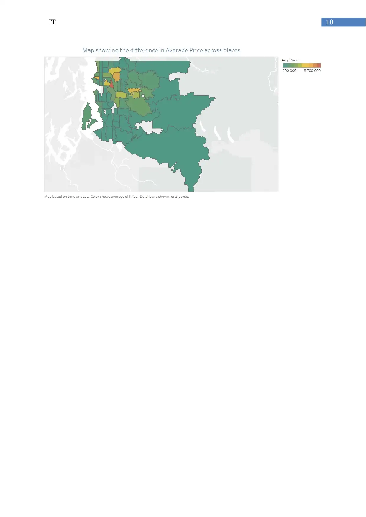
This section presents a representation of the average house prices of the location of
the data. The house prices data contained detailed information of the latitude and longitude of
the houses (Kosara and Mackinlay 2013). The geographical information extracted from the
latitude and longitude of the data provided a geographic map by Tableau. The longitude was
placed in “columns” and latitude in “rows.” To corroborate the latitude and longitude, the zip
code was added as a detail in the chart. Initially the map produced errors due to the default
location of places. However, when the map location was edited to “United States”, the errors
were rectified. In order to delve into the variations in house prices over a geographical
location, the average of the house price (for 2014-15) was used. To gain more information,
the average house prices were colour differentiated. The average price in the range of
2,00,000 was coloured green while 37,000,000 was coloured red. Thus, as the house prices
increases, the range was divided into ten equal sections with changes in depth of the colour.
Thus, from the geomap output, one can easily identify places having very high average price
to very low average prices. From the map, it is seen that at most of the places the average
house prices is around 2,00,000. The map shows that the average house prices is highest at
only one of the shown by red colour. Some of the other places have colours between green
and red.
2.2 GeoMap
This section presents a representation of the average house prices of the location of
the data. The house prices data contained detailed information of the latitude and longitude of
the houses (Kosara and Mackinlay 2013). The geographical information extracted from the
latitude and longitude of the data provided a geographic map by Tableau. The longitude was
placed in “columns” and latitude in “rows.” To corroborate the latitude and longitude, the zip
code was added as a detail in the chart. Initially the map produced errors due to the default
location of places. However, when the map location was edited to “United States”, the errors
were rectified. In order to delve into the variations in house prices over a geographical
location, the average of the house price (for 2014-15) was used. To gain more information,
the average house prices were colour differentiated. The average price in the range of
2,00,000 was coloured green while 37,000,000 was coloured red. Thus, as the house prices
increases, the range was divided into ten equal sections with changes in depth of the colour.
Thus, from the geomap output, one can easily identify places having very high average price
to very low average prices. From the map, it is seen that at most of the places the average
house prices is around 2,00,000. The map shows that the average house prices is highest at
only one of the shown by red colour. Some of the other places have colours between green
and red.
Paraphrase This Document
Need a fresh take? Get an instant paraphrase of this document with our AI Paraphraser
10IT
11IT
References
Fan, C., Xiao, F. and Wang, S., 2014. Development of prediction models for next-day
building energy consumption and peak power demand using data mining techniques. Applied
Energy, 127, pp.1-10.
Kosara, R. and Mackinlay, J., 2013. Storytelling: The next step for visualization. Computer,
46(5), pp.44-50.
Larose, D.T. and Larose, C.D., Exploratory Data Analysis., 2014 Discovering Knowledge in
Data: An Introduction to Data Mining, Second Edition, pp.51-90.
Murphy, S.A., 2013. Data visualization and rapid analytics: applying tableau desktop to
support library decision-making. Journal of Web Librarianship, 7(4), pp.465-476.
Tyrychtr, J., Ulman, M. and Vostrovský, V., 2015. Evaluation of the state of the Business
Intelligence among small Czech farms. Agricultural Economics, 61(2), pp.63-71.
Witten, I.H., Frank, E., Hall, M.A. and Pal, C.J., 2016. Data Mining: Practical machine
learning tools and techniques. Morgan Kaufmann.
Wu, L. and Brynjolfsson, E., 2015. The future of prediction: How Google searches
foreshadow housing prices and sales. In Economic analysis of the digital economy (pp. 89-
118). University of Chicago Press.
Wu, X., Zhu, X., Wu, G.Q. and Ding, W., 2014. Data mining with big data. IEEE
transactions on knowledge and data engineering, 26(1), pp.97-107.
⊘ This is a preview!⊘
Do you want full access?
Subscribe today to unlock all pages.
Trusted by 1+ million students worldwide
1 out of 12
Related Documents


Your All-in-One AI-Powered Toolkit for Academic Success.
+13062052269
info@desklib.com
Available 24*7 on WhatsApp / Email
![[object Object]](/_next/static/media/star-bottom.7253800d.svg)
Unlock your academic potential
Copyright © 2020–2026 A2Z Services. All Rights Reserved. Developed and managed by ZUCOL.