Statistical Analysis of House Prices in Parramatta (2019)
VerifiedAdded on 2023/01/17
|13
|2480
|69
Report
AI Summary
This report presents a statistical analysis of house prices in Parramatta, Australia, from 1999 to 2019. The study investigates factors influencing house prices, including house area, number of bedrooms, bathrooms, and car parking slots. Descriptive statistics reveal trends in house prices, area, and other...
Running head: HOUSES PRICE IN PARRAMATTA
Factors affecting the Houses Price in Parramatta
Name:
Institution:
Factors affecting the Houses Price in Parramatta
Name:
Institution:
Paraphrase This Document
Need a fresh take? Get an instant paraphrase of this document with our AI Paraphraser
HOUSES PRICE IN PARRAMATTA
Executive Summary
The analysis used Parramatta as the primary study region. The main objective of the study
was to determine which factors significantly influence the prices of houses. The research
applied the simple linear regression model to determine whether there was a significant
relationship between selling price and area of the houses. It was established that there was a
significant relationship between house prices and area in square feet. However, the model
explained little about sources of variation (1.7%), which raised questions about model
reliability. One-way ANOVA tests was carried out to determine whether one-bedroom, two-
bedroom and three-bedroom apartments prices were significantly different. Three-bedroom
apartment was found to be economical as it was cheaper than one and two-bedroom
apartment. Lastly, chi-square tests for independence was applied to the data and it established
that there was an association between the number of bedrooms and number of bedrooms.
HOUSES PRICE IN PARRAMATTA
Introduction
The study was determined to determine the sales of houses in the Parramatta, and factors
affecting the sales. Particularly, the primary objective is to determine the sales trend from
1999 to 2019 and identify factors that affect the average sales within this region in Australia.
Factors such as the floor area of the house, number of bedrooms, bathrooms and number of
slots of car parks were considered, and their effect on sales determined. Independence of
factors such as the number of cars park slots and bedrooms was analyzed. Thus, it will be
assessed whether the area in square feet, number of bedrooms and bathrooms, and the slots
available for car parking affect the house sales. The descriptive analysis will help determine
the data distribution, and inferential statistics will help determine the relation of the different
variables, and their effect on the sale price of houses.
Summaries
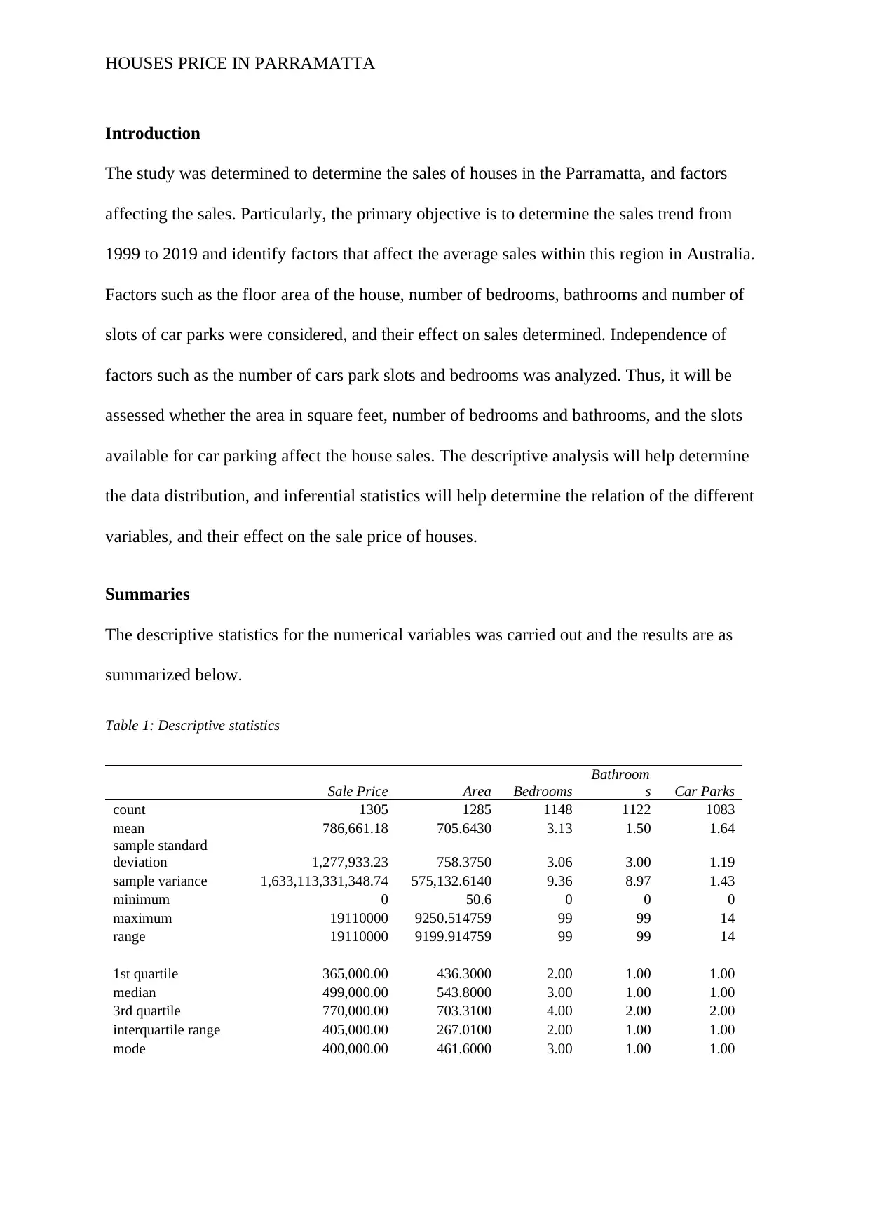
The descriptive statistics for the numerical variables was carried out and the results are as
summarized below.
Table 1: Descriptive statistics
Sale Price Area Bedrooms
Bathroom
s Car Parks
count 1305 1285 1148 1122 1083
mean 786,661.18 705.6430 3.13 1.50 1.64
sample standard
deviation 1,277,933.23 758.3750 3.06 3.00 1.19
sample variance 1,633,113,331,348.74 575,132.6140 9.36 8.97 1.43
minimum 0 50.6 0 0 0
maximum 19110000 9250.514759 99 99 14
range 19110000 9199.914759 99 99 14
1st quartile 365,000.00 436.3000 2.00 1.00 1.00
median 499,000.00 543.8000 3.00 1.00 1.00
3rd quartile 770,000.00 703.3100 4.00 2.00 2.00
interquartile range 405,000.00 267.0100 2.00 1.00 1.00
mode 400,000.00 461.6000 3.00 1.00 1.00
⊘ This is a preview!⊘
Do you want full access?
Subscribe today to unlock all pages.

Trusted by 1+ million students worldwide
HOUSES PRICE IN PARRAMATTA
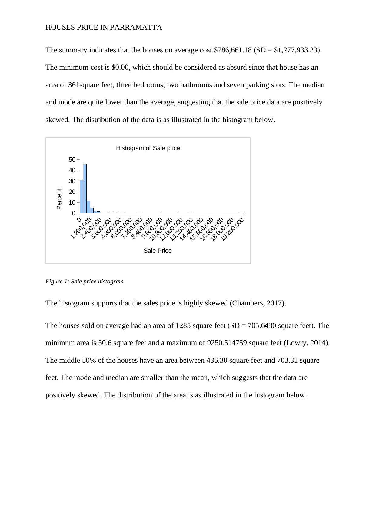
The summary indicates that the houses on average cost $786,661.18 (SD = $1,277,933.23).
The minimum cost is $0.00, which should be considered as absurd since that house has an
area of 361square feet, three bedrooms, two bathrooms and seven parking slots. The median
and mode are quite lower than the average, suggesting that the sale price data are positively
skewed. The distribution of the data is as illustrated in the histogram below.
0
1,200,000
2,400,000
3,600,000
4,800,000
6,000,000
7,200,000
8,400,000
9,600,000
10,800,000
12,000,000
13,200,000
14,400,000
15,600,000
16,800,000
18,000,000
19,200,000
0
10
20
30
40
50
Histogram of Sale price
Sale Price
Percent
Figure 1: Sale price histogram
The histogram supports that the sales price is highly skewed (Chambers, 2017).
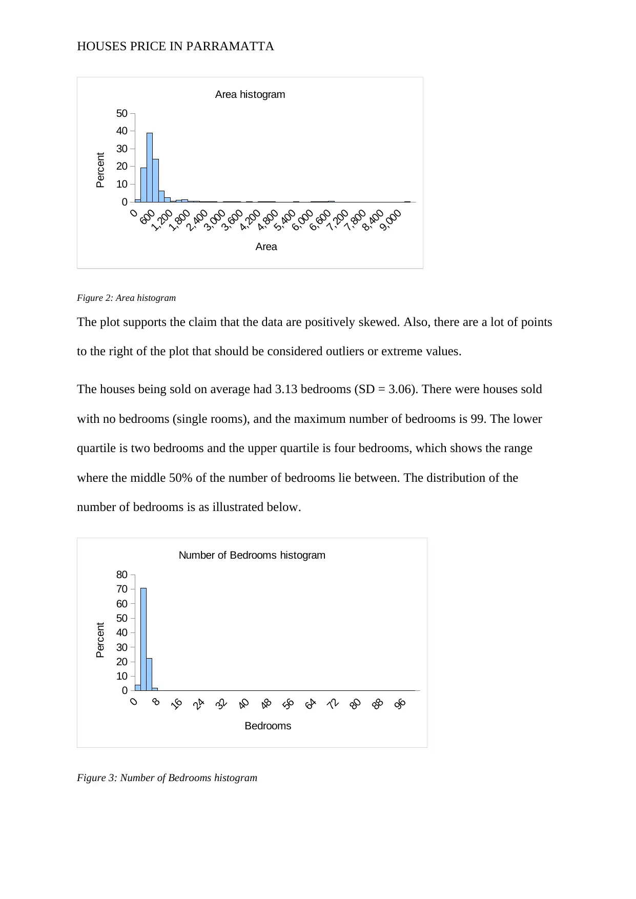
The houses sold on average had an area of 1285 square feet (SD = 705.6430 square feet). The
minimum area is 50.6 square feet and a maximum of 9250.514759 square feet (Lowry, 2014).
The middle 50% of the houses have an area between 436.30 square feet and 703.31 square
feet. The mode and median are smaller than the mean, which suggests that the data are
positively skewed. The distribution of the area is as illustrated in the histogram below.
Paraphrase This Document
Need a fresh take? Get an instant paraphrase of this document with our AI Paraphraser
HOUSES PRICE IN PARRAMATTA
0
600
1,200
1,800
2,400
3,000
3,600
4,200
4,800
5,400
6,000
6,600
7,200
7,800
8,400
9,000
0
10
20
30
40
50
Area histogram
Area
Percent
Figure 2: Area histogram
The plot supports the claim that the data are positively skewed. Also, there are a lot of points
to the right of the plot that should be considered outliers or extreme values.
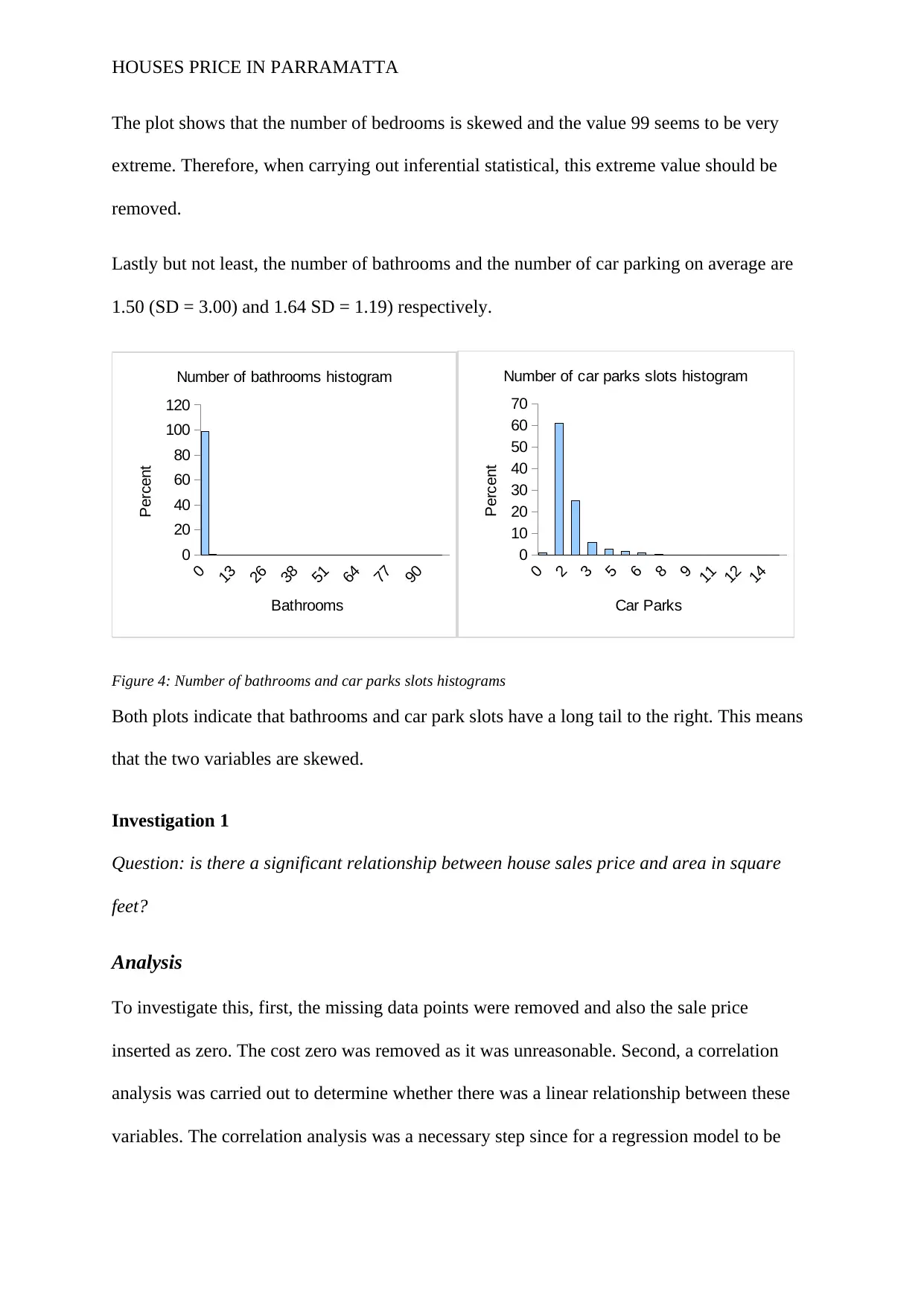
The houses being sold on average had 3.13 bedrooms (SD = 3.06). There were houses sold
with no bedrooms (single rooms), and the maximum number of bedrooms is 99. The lower
quartile is two bedrooms and the upper quartile is four bedrooms, which shows the range
where the middle 50% of the number of bedrooms lie between. The distribution of the
number of bedrooms is as illustrated below.
0
8
16
24
32
40
48
56
64
72
80
88
96
0
10
20
30
40
50
60
70
80
Number of Bedrooms histogram
Bedrooms
Percent
Figure 3: Number of Bedrooms histogram
0
600
1,200
1,800
2,400
3,000
3,600
4,200
4,800
5,400
6,000
6,600
7,200
7,800
8,400
9,000
0
10
20
30
40
50
Area histogram
Area
Percent
Figure 2: Area histogram
The plot supports the claim that the data are positively skewed. Also, there are a lot of points
to the right of the plot that should be considered outliers or extreme values.
The houses being sold on average had 3.13 bedrooms (SD = 3.06). There were houses sold
with no bedrooms (single rooms), and the maximum number of bedrooms is 99. The lower
quartile is two bedrooms and the upper quartile is four bedrooms, which shows the range
where the middle 50% of the number of bedrooms lie between. The distribution of the
number of bedrooms is as illustrated below.
0
8
16
24
32
40
48
56
64
72
80
88
96
0
10
20
30
40
50
60
70
80
Number of Bedrooms histogram
Bedrooms
Percent
Figure 3: Number of Bedrooms histogram
HOUSES PRICE IN PARRAMATTA
The plot shows that the number of bedrooms is skewed and the value 99 seems to be very
extreme. Therefore, when carrying out inferential statistical, this extreme value should be
removed.
Lastly but not least, the number of bathrooms and the number of car parking on average are
1.50 (SD = 3.00) and 1.64 SD = 1.19) respectively.
0
13
26
38
51
64
77
90
0
20
40
60
80
100
120
Number of bathrooms histogram
Bathrooms
Percent
0
2
3
5
6
8
9
11
12
14
0
10
20
30
40
50
60
70
Number of car parks slots histogram
Car Parks
Percent
Figure 4: Number of bathrooms and car parks slots histograms
Both plots indicate that bathrooms and car park slots have a long tail to the right. This means
that the two variables are skewed.
Investigation 1
Question: is there a significant relationship between house sales price and area in square
feet?
Analysis
To investigate this, first, the missing data points were removed and also the sale price
inserted as zero. The cost zero was removed as it was unreasonable. Second, a correlation
analysis was carried out to determine whether there was a linear relationship between these
variables. The correlation analysis was a necessary step since for a regression model to be
⊘ This is a preview!⊘
Do you want full access?
Subscribe today to unlock all pages.

Trusted by 1+ million students worldwide

HOUSES PRICE IN PARRAMATTA
fitted on the data there should be a linear relationship between the dependent and independent
variables (Keller, 2015).
Results
The results are as summarized below.
0
1000
2000
3000
4000
5000
6000
7000
8000
9000
10000
0
5000000
10000000
15000000
20000000
25000000
f(x) = 216.511341059598 x + 627771.561565602
R² = 0.016930471024018
Scatter plot of sales price against house floor area
Area
Sale Price
Figure 5: Scatter plot if house sales price against the floor area
The scatterplot indicates that there is a weak positive association between the floor area of the
house and the sales price (Chambers, 2017). The correlation matrix of the assessment is as
tabulated below.
Table 2: Correlation matrix
Sale Price Area
Sale Price 1.000
Area .130 1.000
1284 sample size
± .055
critical value .05 (two-
tail)
± .072
critical value .01 (two-
tail)
Paraphrase This Document
Need a fresh take? Get an instant paraphrase of this document with our AI Paraphraser

HOUSES PRICE IN PARRAMATTA
The correlation coefficient 0.130 supports that there is a weak positive correlation between
the sale price and the area of the house. This correlation is significant (r (1282) = 0.130, p-
value < .05) (Anderson, Sweeney, Williams, Camm, & Cochran., 2016). Since there exists a
linear relationship, we can fit an ordinal least square (OLS) model that can be used to predict
the sale price of houses in Parramatta. The model summary is as summarized below.
Table 3: regression model summary
r² 0.017 n 1284
r 0.130 k 1
Std. Error 1252216.664 Dep. Var. Sale Price
Regression output confidence interval
variables coefficients std. error t (df=1282) p-value 95% lower 95% upper
Intercept 627,771.5616 47,730.8513 13.152 3.73E-37 534,132.4067 721,410.7165
Area 216.5113 46.0781 4.699 2.90E-06 126.1146 306.9080
Discussion and Conclusion
The fitted regression model is: sale price = 627,771.5616 + 216.5113(area)
The area coefficient is statistically different from zero (β = 216.5113, t (1282) = 4.699, p-
value < .02) (Cohen, West, & Aiken, 2014). This coefficient in a simple way means, when
the floor area increases by one square foot, the sale price is expected to increase by
$216.5113. The coefficient of determination (R-squared) 0.017, indicates that only 1.7% of
sources of variation of the sale price of the houses in Parramatta could be taken into account
by the fitted model. In other words, 98.3% of the variation was not explained by the model
(Keller, 2015). This proportion of variation explained is quite low to ascertain the accuracy of
the values predicted using this model. Further, this means that there are other factors that can
be included in the model to increase the accuracy of the prediction. The other factors may
include, the number of bedrooms, bathrooms or even availability of parking lots.

HOUSES PRICE IN PARRAMATTA
The model indicated that there was enough evidence to conclude that there is a significant
linear relationship between the sale price and the area of the house. However, the model
could only explain a small proportion of variation, which raised the question of the reliability
of the model. Due to the low value of the coefficient of determination, the other factors
should be included in the model to assess whether the model will improve with the addition
of more independent variables. In particular, multiple regression should be fitted to the data.
Investigation 2
Question: Does houses with one bedroom, two bedrooms and three bedrooms’ cost
significantly different?
Analysis
In this case, we are only considering one-bedroom apartment, two bedroom and three-
bedroom apartment and check whether their sales prices are significantly different. If there
exists a significantly different sales price between the different types of apartments, post hoc
analysis should be carried out. In this case, we are comparing three categories of an
independent variable, hence, we use the one-way ANOVA to determine whether the averages
are significantly different.
Results
The test results are as follows:
Table 4: ANOVA test
ANOVA
Source of Variation SS df MS F P-value F crit
Between Groups 1.59443E+13 2 7.97213E+12 8.003616858 0.00036 3.00629
Within Groups 8.48648E+14 852 9.96065E+11
Total 8.64592E+14 854
The results indicate that at least one of the apartment sales price is significantly different
from that of the others (F (2, 852) = 8.00, p-value < .05) (Chatfield, 2018). Therefore, we run
⊘ This is a preview!⊘
Do you want full access?
Subscribe today to unlock all pages.

Trusted by 1+ million students worldwide
HOUSES PRICE IN PARRAMATTA
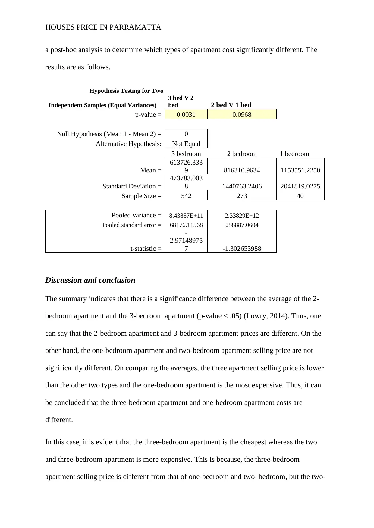
a post-hoc analysis to determine which types of apartment cost significantly different. The
results are as follows.
Hypothesis Testing for Two
Independent Samples (Equal Variances)
3 bed V 2
bed 2 bed V 1 bed
p-value = 0.0031 0.0968
Null Hypothesis (Mean 1 - Mean 2) = 0
Alternative Hypothesis: Not Equal
3 bedroom 2 bedroom 1 bedroom
Mean =
613726.333
9 816310.9634 1153551.2250
Standard Deviation =
473783.003
8 1440763.2406 2041819.0275
Sample Size = 542 273 40
Pooled variance = 8.43857E+11 2.33829E+12
Pooled standard error = 68176.11568 258887.0604
t-statistic =
-
2.97148975
7 -1.302653988
Discussion and conclusion
The summary indicates that there is a significance difference between the average of the 2-
bedroom apartment and the 3-bedroom apartment (p-value < .05) (Lowry, 2014). Thus, one
can say that the 2-bedroom apartment and 3-bedroom apartment prices are different. On the
other hand, the one-bedroom apartment and two-bedroom apartment selling price are not
significantly different. On comparing the averages, the three apartment selling price is lower
than the other two types and the one-bedroom apartment is the most expensive. Thus, it can
be concluded that the three-bedroom apartment and one-bedroom apartment costs are
different.
In this case, it is evident that the three-bedroom apartment is the cheapest whereas the two
and three-bedroom apartment is more expensive. This is because, the three-bedroom
apartment selling price is different from that of one-bedroom and two–bedroom, but the two-
Paraphrase This Document
Need a fresh take? Get an instant paraphrase of this document with our AI Paraphraser

HOUSES PRICE IN PARRAMATTA
bedroom and one-bedroom apartment are not significantly different. Thus, if an individual is
planning on purchasing a new apartment it is highly recommended he/she purchase a three-
bedroom apartment. However, in case of further analysis, it is important to take into account
other factors that might be affecting the cost of a house such as nearness to the city, street
among others.
Investigation 3
Question: are the number of bedrooms and bathrooms independent?
Analysis
In this case, we are interested to determine whether the number of bedrooms and number of
bathrooms in a house for sale is associated. Consequently, we carry out chi-square for
independence to test the hypothesis: H0: the number of bedrooms and bathrooms are
independent versus Ha: the number of bedrooms and bathrooms are not independent.
Results
The summary of the results is as tabulated below.
0 1 2 3 4 5 6 11
0
50
100
150
200
250
300
350
400
450
Clustered bar chart for bathrooms and bedrooms
0
1
2
3
4
5
6
7
8
9
10
11
13
Bathrooms
Frequency
Table 5: Clustered column chart of Bedrooms and bathrooms’ distribution
HOUSES PRICE IN PARRAMATTA
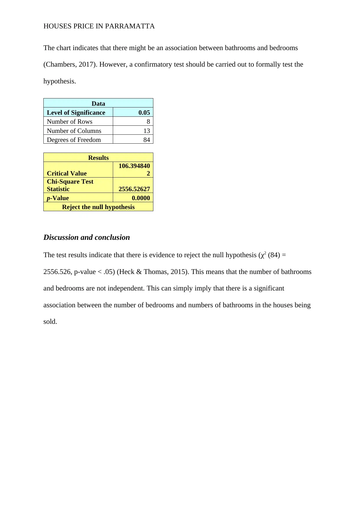
The chart indicates that there might be an association between bathrooms and bedrooms
(Chambers, 2017). However, a confirmatory test should be carried out to formally test the
hypothesis.
Data
Level of Significance 0.05
Number of Rows 8
Number of Columns 13
Degrees of Freedom 84
Results
Critical Value
106.394840
2
Chi-Square Test
Statistic 2556.52627
p-Value 0.0000
Reject the null hypothesis
Discussion and conclusion
The test results indicate that there is evidence to reject the null hypothesis (χ2 (84) =
2556.526, p-value < .05) (Heck & Thomas, 2015). This means that the number of bathrooms
and bedrooms are not independent. This can simply imply that there is a significant
association between the number of bedrooms and numbers of bathrooms in the houses being
sold.
⊘ This is a preview!⊘
Do you want full access?
Subscribe today to unlock all pages.

Trusted by 1+ million students worldwide
HOUSES PRICE IN PARRAMATTA
References
Anderson, D. R., Sweeney, D. J., Williams, T. A., Camm, J. D., & Cochran., J. J. (2016).
Statistics for business & economics (13th ed.). Nelson Education.
Chambers, J. M. (2017). Graphical Methods for Data Analysis: 0. Chapman and Hall/CRC.
Chatfield, C. (2018). Statistics for technology: a course in applied statistics (3rd Edition ed.).
New York: Routledge.
Cohen, P., West, S. G., & Aiken, L. S. (2014). Applied multiple regression/correlation
analysis for the behavioral sciences (2nd ed.). Psychology Press.
Heck, R. H., & Thomas, S. L. (2015). An introduction to multilevel modeling techniques;
MLM and SEM approaches using Mplus. Routledge.
Keller, G. (2015). Statistics for Management and Economics, Abbreviated. Cengage
Learning.
Lowry, R. (2014). Concepts and applications of inferential statistics.
Sullivan III, M. (2015). Fundamentals of statistics. Pearson.
1 out of 13
Your All-in-One AI-Powered Toolkit for Academic Success.
+13062052269
info@desklib.com
Available 24*7 on WhatsApp / Email
![[object Object]](/_next/static/media/star-bottom.7253800d.svg)
Unlock your academic potential
© 2024 | Zucol Services PVT LTD | All rights reserved.


