Estimating Cost of Debt (kd): Historical Data, T-Security's Yield Curve, and Bond Yield

This article discusses three approaches to estimate the cost of debt (kd) for a company: using historical data, T-security's yield curve, and bond yield. It explains the steps involved in each approach and highlights the limitations of historical data. The article also provides a calculation example for the cost of capital of a company based on different factors.

How should we estimate cost of debt (kd)?
Approach 1: Use historical data [Bank loan- it is more applicable for bank loan. There is no
secondary market for bank loan]
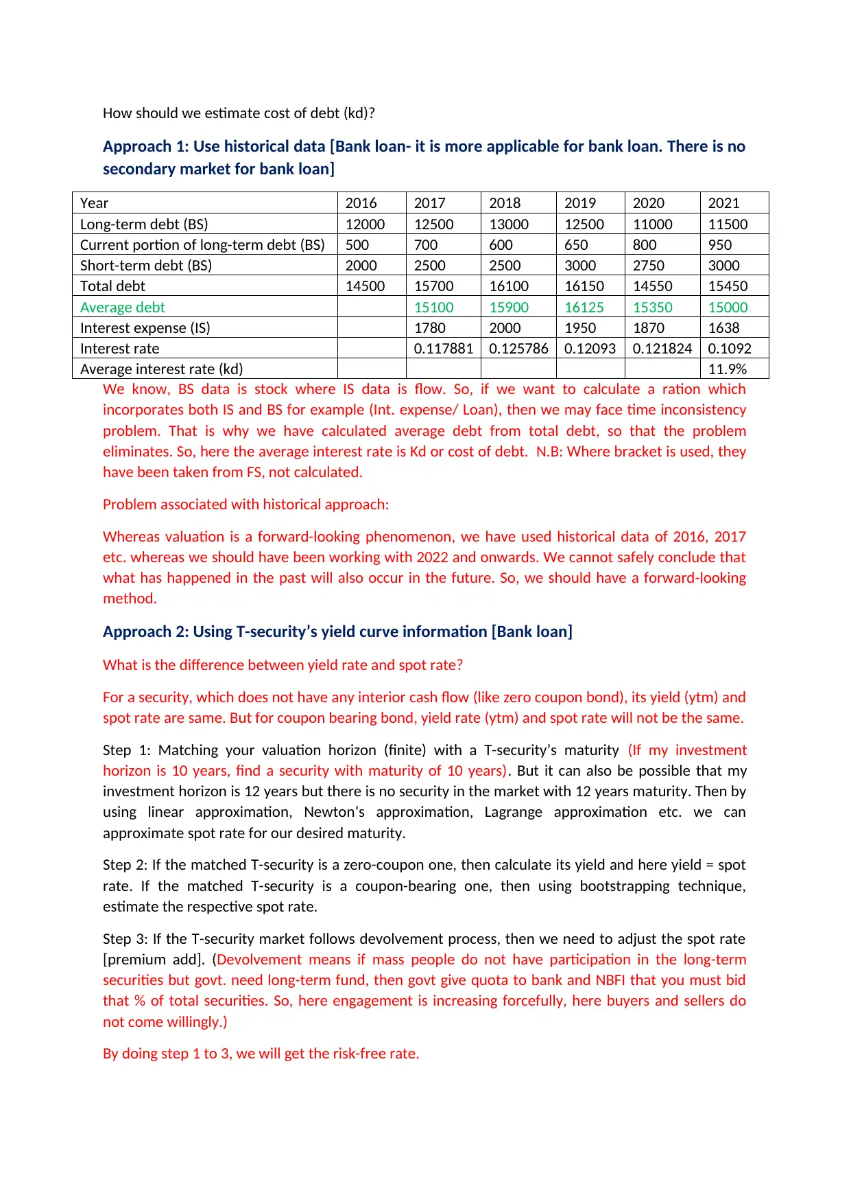
Year 2016 2017 2018 2019 2020 2021
Long-term debt (BS) 12000 12500 13000 12500 11000 11500
Current portion of long-term debt (BS) 500 700 600 650 800 950
Short-term debt (BS) 2000 2500 2500 3000 2750 3000
Total debt 14500 15700 16100 16150 14550 15450
Average debt 15100 15900 16125 15350 15000
Interest expense (IS) 1780 2000 1950 1870 1638
Interest rate 0.117881 0.125786 0.12093 0.121824 0.1092
Average interest rate (kd) 11.9%
We know, BS data is stock where IS data is flow. So, if we want to calculate a ration which
incorporates both IS and BS for example (Int. expense/ Loan), then we may face time inconsistency
problem. That is why we have calculated average debt from total debt, so that the problem
eliminates. So, here the average interest rate is Kd or cost of debt. N.B: Where bracket is used, they
have been taken from FS, not calculated.
Problem associated with historical approach:
Whereas valuation is a forward-looking phenomenon, we have used historical data of 2016, 2017
etc. whereas we should have been working with 2022 and onwards. We cannot safely conclude that
what has happened in the past will also occur in the future. So, we should have a forward-looking
method.
Approach 2: Using T-security’s yield curve information [Bank loan]
What is the difference between yield rate and spot rate?
For a security, which does not have any interior cash flow (like zero coupon bond), its yield (ytm) and
spot rate are same. But for coupon bearing bond, yield rate (ytm) and spot rate will not be the same.
Step 1: Matching your valuation horizon (finite) with a T-security’s maturity (If my investment
horizon is 10 years, find a security with maturity of 10 years). But it can also be possible that my
investment horizon is 12 years but there is no security in the market with 12 years maturity. Then by
using linear approximation, Newton’s approximation, Lagrange approximation etc. we can
approximate spot rate for our desired maturity.
Step 2: If the matched T-security is a zero-coupon one, then calculate its yield and here yield = spot
rate. If the matched T-security is a coupon-bearing one, then using bootstrapping technique,
estimate the respective spot rate.
Step 3: If the T-security market follows devolvement process, then we need to adjust the spot rate
[premium add]. (Devolvement means if mass people do not have participation in the long-term
securities but govt. need long-term fund, then govt give quota to bank and NBFI that you must bid
that % of total securities. So, here engagement is increasing forcefully, here buyers and sellers do
not come willingly.)
By doing step 1 to 3, we will get the risk-free rate.

Step 4: Then track your firm’s credit rating and also track the yield spread. Yield spread is an
indicator of your firm’s credit riskiness. (Yield spread is the difference of spread between a risk-free
firm and risky firm)
Step 5: Cost of debt = Spot rate + yield spread
Approach 3: Bond yield [existing bond]
Then the whole process becomes very simple. We will then calculate the YTM since we know the
price of the bond, payment structure, coupon amount, maturity.
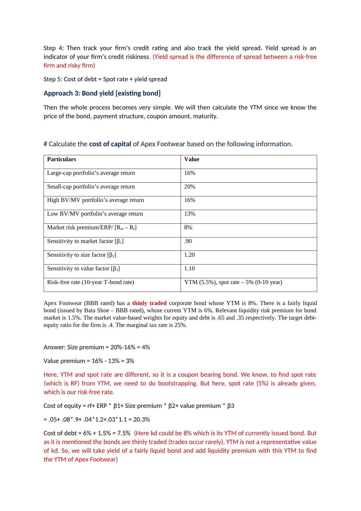
# Calculate the cost of capital of Apex Footwear based on the following information.
Particulars Value
Large-cap portfolio’s average return 16%
Small-cap portfolio’s average return 20%
High BV/MV portfolio’s average return 16%
Low BV/MV portfolio’s average return 13%
Market risk premium/ERP/ [Rm – Rf] 8%
Sensitivity to market factor [β1] .90
Sensitivity to size factor [β2] 1.20
Sensitivity to value factor [β3] 1.10
Risk-free rate (10-year T-bond rate) YTM (5.5%), spot rate – 5% (0-10 year)
Apex Footwear (BBB rated) has a thinly traded corporate bond whose YTM is 8%. There is a fairly liquid
bond (issued by Bata Shoe – BBB rated), whose current YTM is 6%. Relevant liquidity risk premium for bond
market is 1.5%. The market value-based weights for equity and debt is .65 and .35 respectively. The target debt-
equity ratio for the firm is .4. The marginal tax rate is 25%.
Answer: Size premium = 20%-16% = 4%
Value premium = 16% - 13% = 3%
Here, YTM and spot rate are different, so it is a coupon bearing bond. We know, to find spot rate
(which is RF) from YTM, we need to do bootstrapping. But here, spot rate (5%) is already given,
which is our risk-free rate.
Cost of equity = rf+ ERP * β1+ Size premium * β2+ value premium * β3
= .05+ .08*.9+ .04*1.2+.03*1.1 = 20.3%
Cost of debt = 6% + 1.5% = 7.5% (Here kd could be 8% which is its YTM of currently issued bond. But
as it is mentioned the bonds are thinly traded (trades occur rarely), YTM is not a representative value
of kd. So, we will take yield of a fairly liquid bond and add liquidity premium with this YTM to find
the YTM of Apex Footwear)

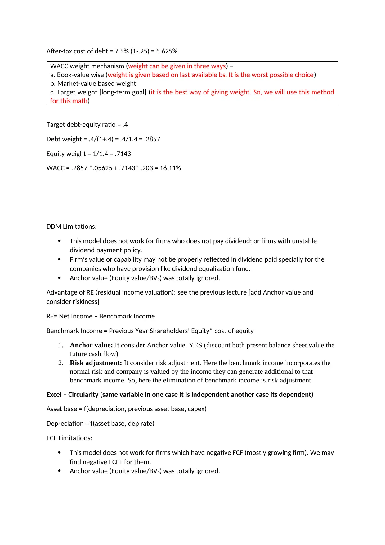
After-tax cost of debt = 7.5% (1-.25) = 5.625%
WACC weight mechanism (weight can be given in three ways) –
a. Book-value wise (weight is given based on last available bs. It is the worst possible choice)
b. Market-value based weight
c. Target weight [long-term goal] (it is the best way of giving weight. So, we will use this method
for this math)
Target debt-equity ratio = .4
Debt weight = .4/(1+.4) = .4/1.4 = .2857
Equity weight = 1/1.4 = .7143
WACC = .2857 *.05625 + .7143* .203 = 16.11%
DDM Limitations:
 This model does not work for firms who does not pay dividend; or firms with unstable
dividend payment policy.
 Firm’s value or capability may not be properly reflected in dividend paid specially for the
companies who have provision like dividend equalization fund.
 Anchor value (Equity value/BV0) was totally ignored.
Advantage of RE (residual income valuation): see the previous lecture [add Anchor value and
consider riskiness]
RE= Net Income – Benchmark Income
Benchmark Income = Previous Year Shareholders’ Equity* cost of equity
1. Anchor value: It consider Anchor value. YES (discount both present balance sheet value the
future cash flow)
2. Risk adjustment: It consider risk adjustment. Here the benchmark income incorporates the
normal risk and company is valued by the income they can generate additional to that
benchmark income. So, here the elimination of benchmark income is risk adjustment
Excel – Circularity (same variable in one case it is independent another case its dependent)
Asset base = f(depreciation, previous asset base, capex)
Depreciation = f(asset base, dep rate)
FCF Limitations:
 This model does not work for firms which have negative FCF (mostly growing firm). We may
find negative FCFF for them.
 Anchor value (Equity value/BV0) was totally ignored.