Assignment on the Importance of Hydro graph
VerifiedAdded on 2022/09/28
|15
|2769
|23
Assignment
AI Summary
Contribute Materials
Your contribution can guide someone’s learning journey. Share your
documents today.
Introduction
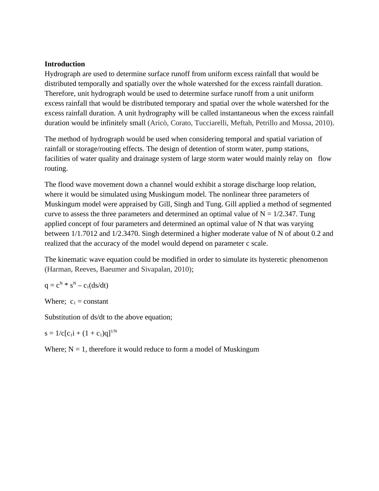
Hydrograph are used to determine surface runoff from uniform excess rainfall that would be
distributed temporally and spatially over the whole watershed for the excess rainfall duration.
Therefore, unit hydrograph would be used to determine surface runoff from a unit uniform
excess rainfall that would be distributed temporary and spatial over the whole watershed for the
excess rainfall duration. A unit hydrography will be called instantaneous when the excess rainfall
duration would be infinitely small (Aricò, Corato, Tucciarelli, Meftah, Petrillo and Mossa, 2010).
The method of hydrograph would be used when considering temporal and spatial variation of
rainfall or storage/routing effects. The design of detention of storm water, pump stations,
facilities of water quality and drainage system of large storm water would mainly relay on flow
routing.
The flood wave movement down a channel would exhibit a storage discharge loop relation,
where it would be simulated using Muskingum model. The nonlinear three parameters of
Muskingum model were appraised by Gill, Singh and Tung. Gill applied a method of segmented
curve to assess the three parameters and determined an optimal value of N = 1/2.347. Tung
applied concept of four parameters and determined an optimal value of N that was varying
between 1/1.7012 and 1/2.3470. Singh determined a higher moderate value of N of about 0.2 and
realized that the accuracy of the model would depend on parameter c scale.
The kinematic wave equation could be modified in order to simulate its hysteretic phenomenon
(Harman, Reeves, Baeumer and Sivapalan, 2010);
q = cN * sN – c1(ds/dt)
Where; c1 = constant
Substitution of ds/dt to the above equation;
s = 1/c[c1i + (1 + c1)q]1/N
Where; N = 1, therefore it would reduce to form a model of Muskingum
Secure Best Marks with AI Grader
Need help grading? Try our AI Grader for instant feedback on your assignments.
Terms used in determine unit flow rate
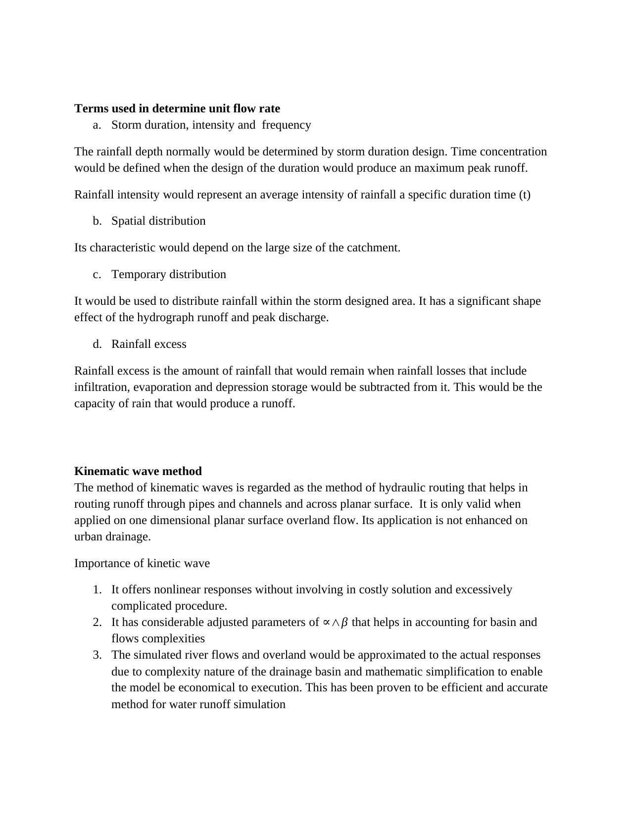
a. Storm duration, intensity and frequency
The rainfall depth normally would be determined by storm duration design. Time concentration
would be defined when the design of the duration would produce an maximum peak runoff.
Rainfall intensity would represent an average intensity of rainfall a specific duration time (t)
b. Spatial distribution
Its characteristic would depend on the large size of the catchment.
c. Temporary distribution
It would be used to distribute rainfall within the storm designed area. It has a significant shape
effect of the hydrograph runoff and peak discharge.
d. Rainfall excess
Rainfall excess is the amount of rainfall that would remain when rainfall losses that include
infiltration, evaporation and depression storage would be subtracted from it. This would be the
capacity of rain that would produce a runoff.
Kinematic wave method
The method of kinematic waves is regarded as the method of hydraulic routing that helps in
routing runoff through pipes and channels and across planar surface. It is only valid when
applied on one dimensional planar surface overland flow. Its application is not enhanced on
urban drainage.
Importance of kinetic wave
1. It offers nonlinear responses without involving in costly solution and excessively
complicated procedure.
2. It has considerable adjusted parameters of ∝∧β that helps in accounting for basin and
flows complexities
3. The simulated river flows and overland would be approximated to the actual responses
due to complexity nature of the drainage basin and mathematic simplification to enable
the model be economical to execution. This has been proven to be efficient and accurate
method for water runoff simulation
The features of kinematic wave would dominate dynamic wave considering flows having less
Froude number than or equal to 2 (F ≤ 2).
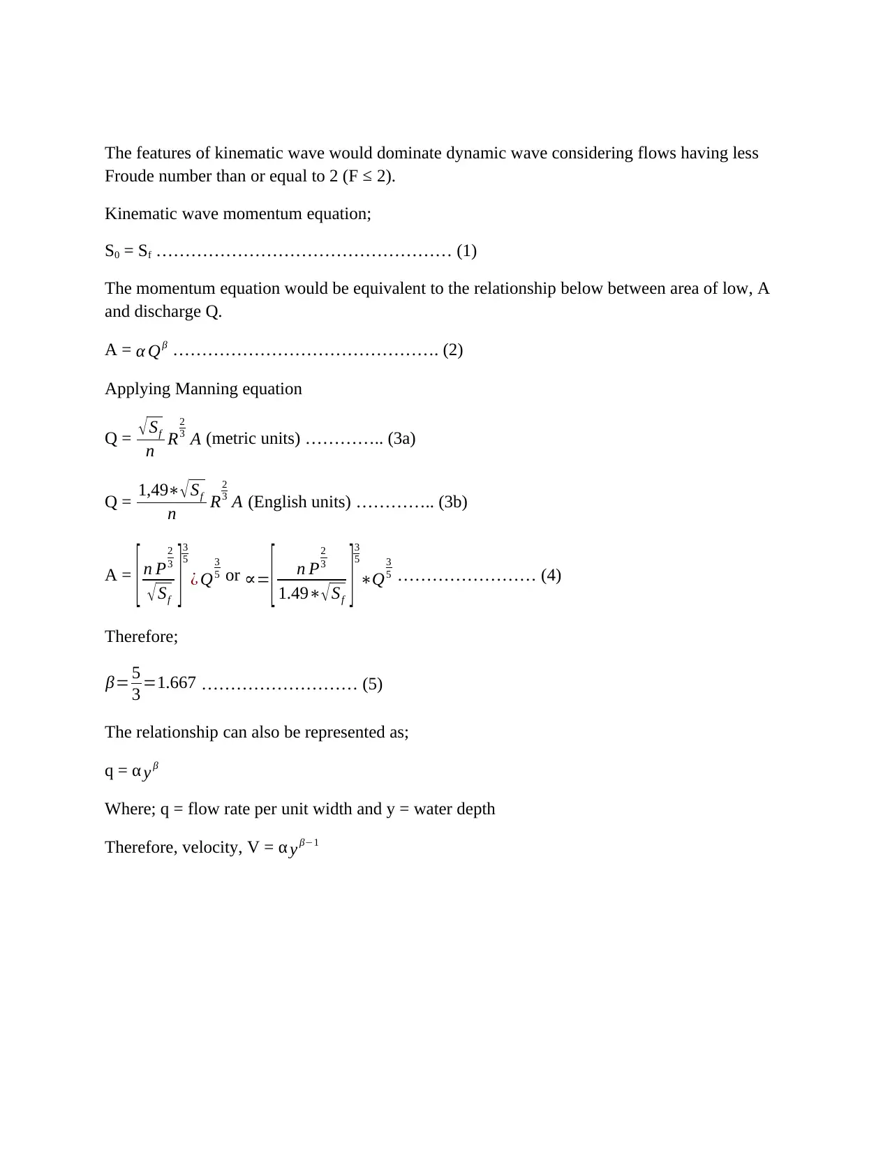
Kinematic wave momentum equation;
S0 = Sf …………………………………………… (1)
The momentum equation would be equivalent to the relationship below between area of low, A
and discharge Q.
A = α Qβ ………………………………………. (2)
Applying Manning equation
Q = √Sf
n R
2
3 A (metric units) ………….. (3a)
Q = 1,49∗√Sf
n R
2
3 A (English units) ………….. (3b)
A = [ n P
2
3
√Sf ]3
5
¿ Q
3
5 or ∝= [ n P
2
3
1.49∗√Sf ]3
5
∗Q
3
5 …………………… (4)
Therefore;
β= 5
3 =1.667 ……………………… (5)
The relationship can also be represented as;
q = α y β
Where; q = flow rate per unit width and y = water depth
Therefore, velocity, V = α y β−1
Calculations
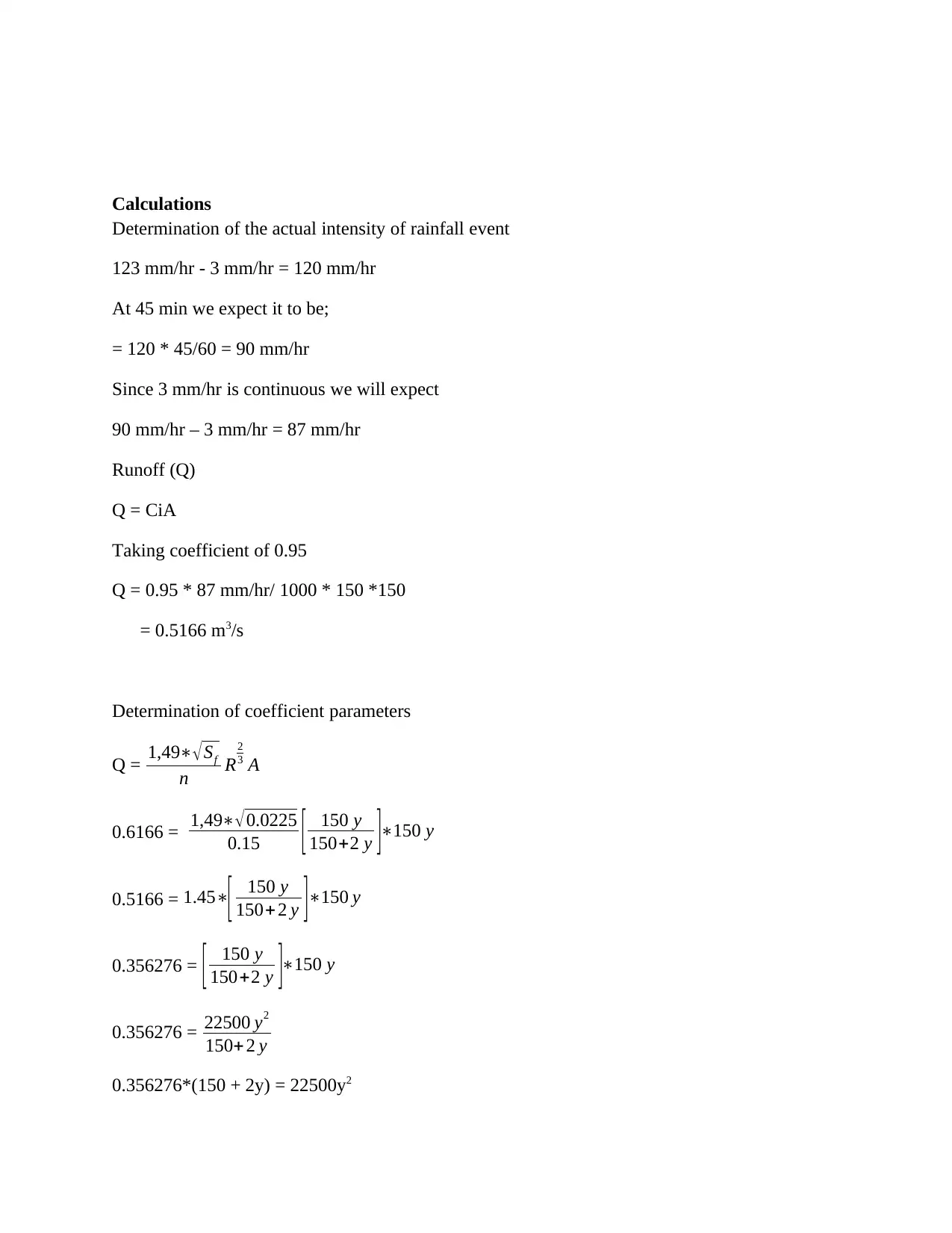
Determination of the actual intensity of rainfall event
123 mm/hr - 3 mm/hr = 120 mm/hr
At 45 min we expect it to be;
= 120 * 45/60 = 90 mm/hr
Since 3 mm/hr is continuous we will expect
90 mm/hr – 3 mm/hr = 87 mm/hr
Runoff (Q)
Q = CiA
Taking coefficient of 0.95
Q = 0.95 * 87 mm/hr/ 1000 * 150 *150
= 0.5166 m3/s
Determination of coefficient parameters
Q = 1,49∗√Sf
n R
2
3 A
0.6166 = 1,49∗√ 0.0225
0.15 [ 150 y
150+2 y ]∗150 y
0.5166 = 1.45∗
[ 150 y
150+ 2 y ]∗150 y
0.356276 = [ 150 y
150+2 y ]∗150 y
0.356276 = 22500 y2
150+ 2 y
0.356276*(150 + 2y) = 22500y2
Secure Best Marks with AI Grader
Need help grading? Try our AI Grader for instant feedback on your assignments.
53.4414 + 0.712552y = 22500y2
22500y2 – 0.712552y -53.4414 = 0
Y = 0.0487516 m
∝= [ 0.15∗150
2
3
1.49∗√0.0225 ]3
5
∝= [ n P
2
3
1.49∗√Sf ]3
5
= 5.842
Therefore, β= 5
3 =1.667
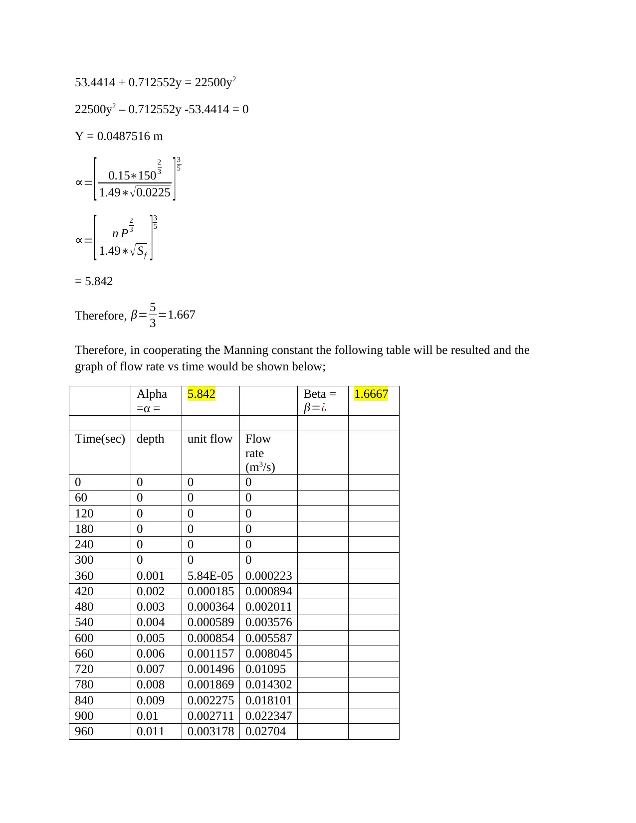
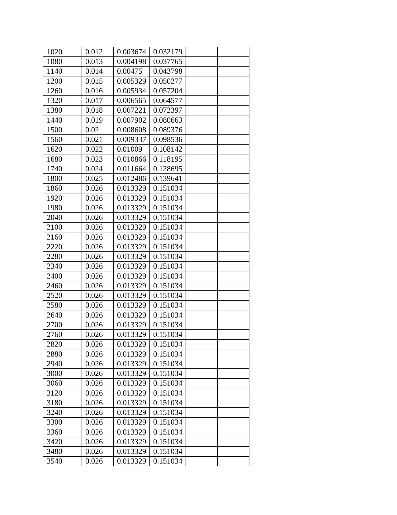
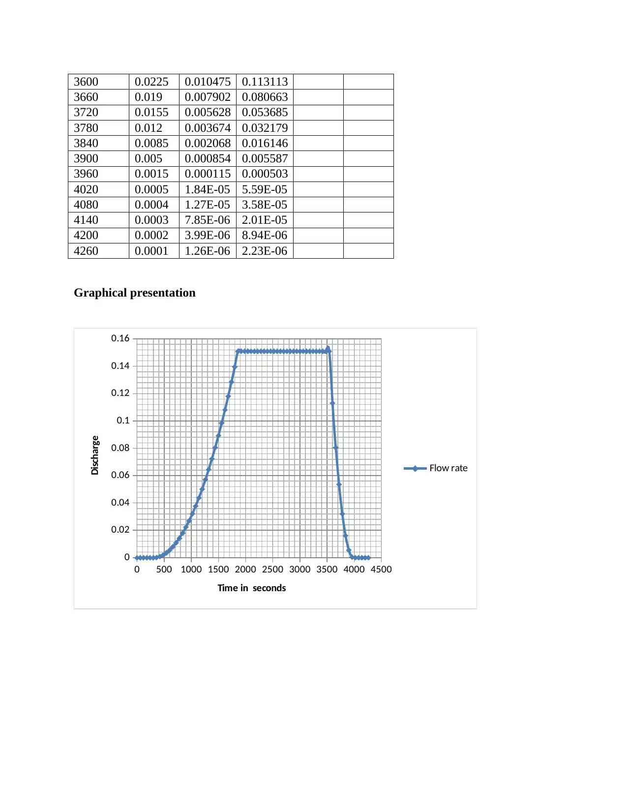
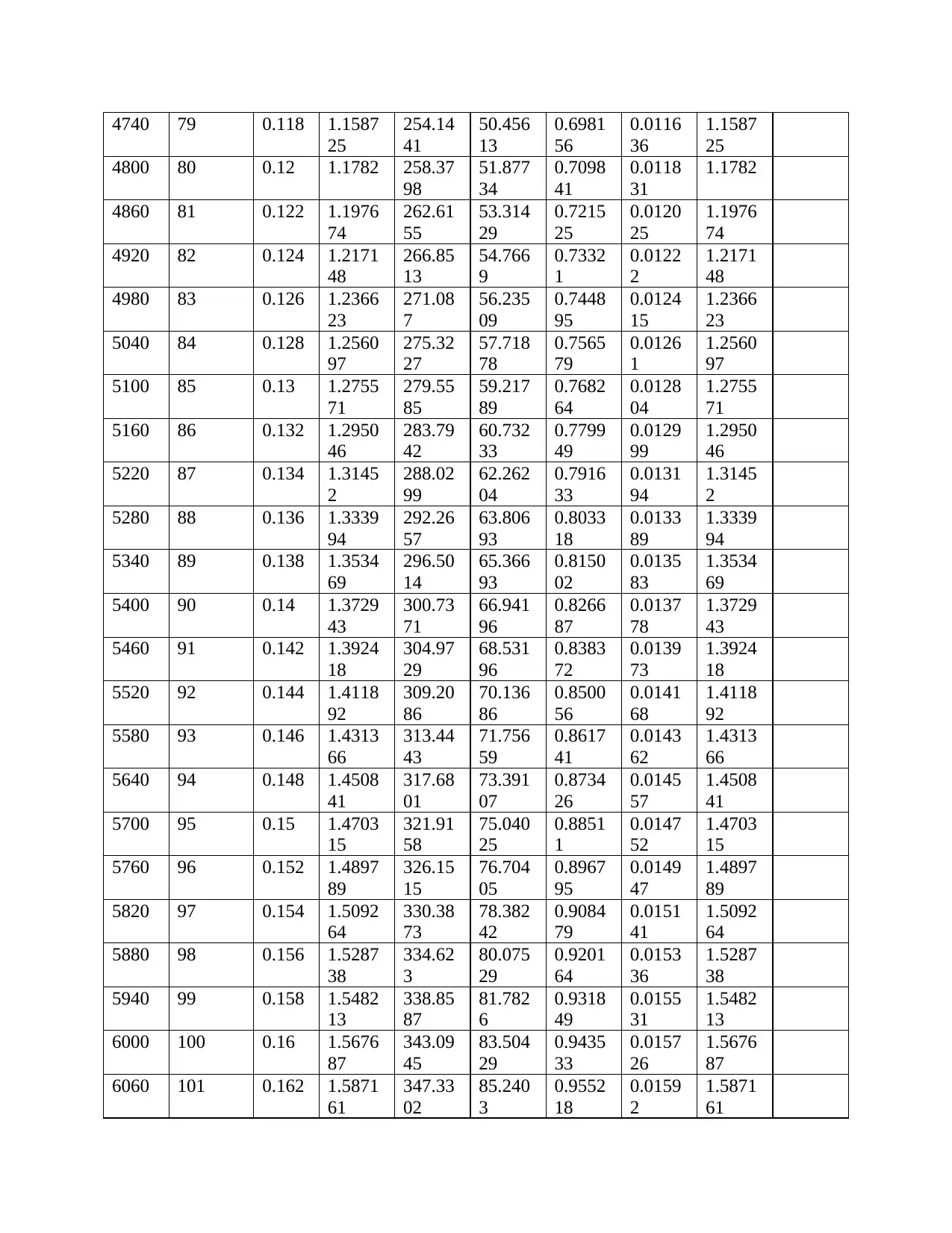
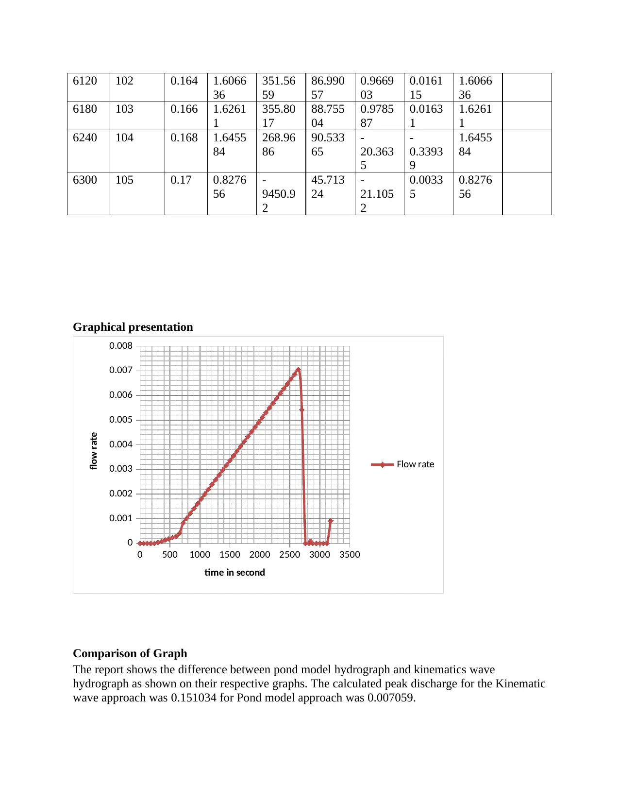
Therefore, in cooperating the Manning constant the following table will be resulted and the
graph of flow rate vs time would be shown below;
Alpha
=α =
5.842 Beta =
β=¿
1.6667
Time(sec) depth unit flow Flow
rate
(m3/s)
0 0 0 0
60 0 0 0
120 0 0 0
180 0 0 0
240 0 0 0
300 0 0 0
360 0.001 5.84E-05 0.000223
420 0.002 0.000185 0.000894
480 0.003 0.000364 0.002011
540 0.004 0.000589 0.003576
600 0.005 0.000854 0.005587
660 0.006 0.001157 0.008045
720 0.007 0.001496 0.01095
780 0.008 0.001869 0.014302
840 0.009 0.002275 0.018101
900 0.01 0.002711 0.022347
960 0.011 0.003178 0.02704
1020 0.012 0.003674 0.032179
1080 0.013 0.004198 0.037765
1140 0.014 0.00475 0.043798
1200 0.015 0.005329 0.050277
1260 0.016 0.005934 0.057204
1320 0.017 0.006565 0.064577
1380 0.018 0.007221 0.072397
1440 0.019 0.007902 0.080663
1500 0.02 0.008608 0.089376
1560 0.021 0.009337 0.098536
1620 0.022 0.01009 0.108142
1680 0.023 0.010866 0.118195
1740 0.024 0.011664 0.128695
1800 0.025 0.012486 0.139641
1860 0.026 0.013329 0.151034
1920 0.026 0.013329 0.151034
1980 0.026 0.013329 0.151034
2040 0.026 0.013329 0.151034
2100 0.026 0.013329 0.151034
2160 0.026 0.013329 0.151034
2220 0.026 0.013329 0.151034
2280 0.026 0.013329 0.151034
2340 0.026 0.013329 0.151034
2400 0.026 0.013329 0.151034
2460 0.026 0.013329 0.151034
2520 0.026 0.013329 0.151034
2580 0.026 0.013329 0.151034
2640 0.026 0.013329 0.151034
2700 0.026 0.013329 0.151034
2760 0.026 0.013329 0.151034
2820 0.026 0.013329 0.151034
2880 0.026 0.013329 0.151034
2940 0.026 0.013329 0.151034
3000 0.026 0.013329 0.151034
3060 0.026 0.013329 0.151034
3120 0.026 0.013329 0.151034
3180 0.026 0.013329 0.151034
3240 0.026 0.013329 0.151034
3300 0.026 0.013329 0.151034
3360 0.026 0.013329 0.151034
3420 0.026 0.013329 0.151034
3480 0.026 0.013329 0.151034
3540 0.026 0.013329 0.151034
3600 0.0225 0.010475 0.113113
3660 0.019 0.007902 0.080663
3720 0.0155 0.005628 0.053685
3780 0.012 0.003674 0.032179
3840 0.0085 0.002068 0.016146
3900 0.005 0.000854 0.005587
3960 0.0015 0.000115 0.000503
4020 0.0005 1.84E-05 5.59E-05
4080 0.0004 1.27E-05 3.58E-05
4140 0.0003 7.85E-06 2.01E-05
4200 0.0002 3.99E-06 8.94E-06
4260 0.0001 1.26E-06 2.23E-06
Graphical presentation
0 500 1000 1500 2000 2500 3000 3500 4000 4500
0
0.02
0.04
0.06
0.08
0.1
0.12
0.14
0.16
Flow rate
Time in seconds
Discharge
Paraphrase This Document
Need a fresh take? Get an instant paraphrase of this document with our AI Paraphraser
Pond model method
The runoff routing hydrograph using detention pond models would depend on the size of the
respective pond in APSWM. The representation of storage characteristic discharge would be
similar to that used on conventional storm water. The application of mathematical concepts
would help in derivation of analytical expression form of distribution frequency of a peak
outflow downstream from a detention pond (Glenn and Bartell, 2010).
Probabilistic detention pond flood routing
If there is a detention pond upstream of a detention pond
under study, as shown schematically in Fig. 2, the effect of
the upstream detention pond may be taken into account by
modifying the parameters of the catchment draining into the
downstream detention pond. However, this needs to be done
properly to ensure that the flood routing effect of the up-
stream pond is recognized and represented as accurately and
explicitly as possible. In essence, catchments transform the
Detention pond flood routing
The presence of upstream detention pond would lead to modification of the catchment draining
parameters in the downstream retention pond. The process requires attention to ensure accuracy
and explicitly of the recognized upstream effect of the flood routing.
The peak of attenuation would depend on the time of concentration, where a small time of
concentration would lead to a lower degree of attenuation. The consideration of detention pond’s
outflow hydrograph to be approximated as a triangle would help in accountability of reduced
flood peak effect by increasing concentration time of the upstream that would be discharged into
the pond.
Calculations
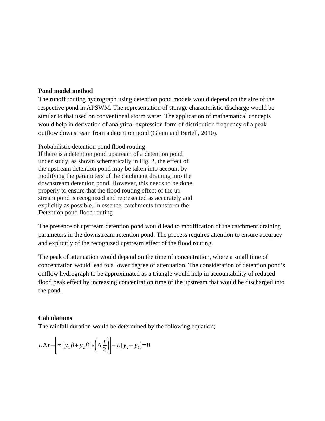
The rainfall duration would be determined by the following equation;
L ∆ t−
[∝ ( y1 β + y2 β )∗(∆ t
2 ) ]−L ( y2− y1 ) =0
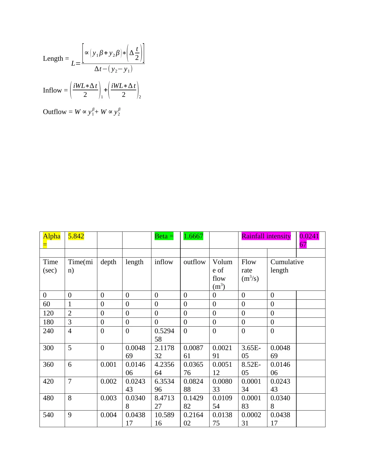
Length = L= [ ∝ ( y1 β + y2 β )∗( ∆ t
2 ) ]
∆t−( y2− y1 )
Inflow = ( iWL∗∆ t
2 )1
+( iWL∗∆ t
2 )2
Outflow = W ∝ y1
β+ W ∝ y2
β
Alpha
=
5.842 Beta = 1.6667 Rainfall intensity 0.0241
67
Time
(sec)
Time(mi
n)
depth length inflow outflow Volum
e of
flow
(m3)
Flow
rate
(m3/s)
Cumulative
length
0 0 0 0 0 0 0 0 0
60 1 0 0 0 0 0 0 0
120 2 0 0 0 0 0 0 0
180 3 0 0 0 0 0 0 0
240 4 0 0 0.5294
58
0 0 0 0
300 5 0 0.0048
69
2.1178
32
0.0087
61
0.0021
91
3.65E-
05
0.0048
69
360 6 0.001 0.0146
06
4.2356
64
0.0365
76
0.0051
12
8.52E-
05
0.0146
06
420 7 0.002 0.0243
43
6.3534
96
0.0824
88
0.0080
33
0.0001
34
0.0243
43
480 8 0.003 0.0340
8
8.4713
27
0.1429
82
0.0109
54
0.0001
83
0.0340
8
540 9 0.004 0.0438
17
10.589
16
0.2164
02
0.0138
75
0.0002
31
0.0438
17
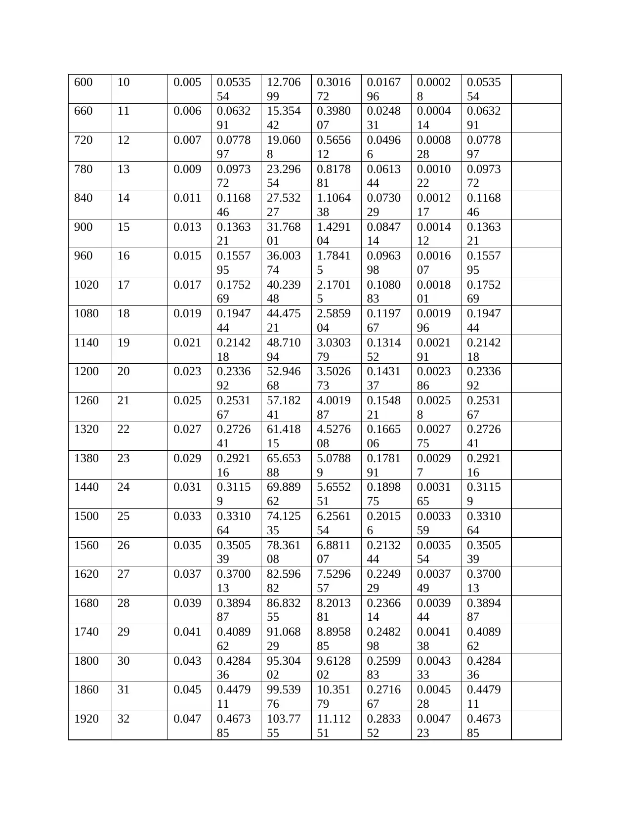
600 10 0.005 0.0535
54
12.706
99
0.3016
72
0.0167
96
0.0002
8
0.0535
54
660 11 0.006 0.0632
91
15.354
42
0.3980
07
0.0248
31
0.0004
14
0.0632
91
720 12 0.007 0.0778
97
19.060
8
0.5656
12
0.0496
6
0.0008
28
0.0778
97
780 13 0.009 0.0973
72
23.296
54
0.8178
81
0.0613
44
0.0010
22
0.0973
72
840 14 0.011 0.1168
46
27.532
27
1.1064
38
0.0730
29
0.0012
17
0.1168
46
900 15 0.013 0.1363
21
31.768
01
1.4291
04
0.0847
14
0.0014
12
0.1363
21
960 16 0.015 0.1557
95
36.003
74
1.7841
5
0.0963
98
0.0016
07
0.1557
95
1020 17 0.017 0.1752
69
40.239
48
2.1701
5
0.1080
83
0.0018
01
0.1752
69
1080 18 0.019 0.1947
44
44.475
21
2.5859
04
0.1197
67
0.0019
96
0.1947
44
1140 19 0.021 0.2142
18
48.710
94
3.0303
79
0.1314
52
0.0021
91
0.2142
18
1200 20 0.023 0.2336
92
52.946
68
3.5026
73
0.1431
37
0.0023
86
0.2336
92
1260 21 0.025 0.2531
67
57.182
41
4.0019
87
0.1548
21
0.0025
8
0.2531
67
1320 22 0.027 0.2726
41
61.418
15
4.5276
08
0.1665
06
0.0027
75
0.2726
41
1380 23 0.029 0.2921
16
65.653
88
5.0788
9
0.1781
91
0.0029
7
0.2921
16
1440 24 0.031 0.3115
9
69.889
62
5.6552
51
0.1898
75
0.0031
65
0.3115
9
1500 25 0.033 0.3310
64
74.125
35
6.2561
54
0.2015
6
0.0033
59
0.3310
64
1560 26 0.035 0.3505
39
78.361
08
6.8811
07
0.2132
44
0.0035
54
0.3505
39
1620 27 0.037 0.3700
13
82.596
82
7.5296
57
0.2249
29
0.0037
49
0.3700
13
1680 28 0.039 0.3894
87
86.832
55
8.2013
81
0.2366
14
0.0039
44
0.3894
87
1740 29 0.041 0.4089
62
91.068
29
8.8958
85
0.2482
98
0.0041
38
0.4089
62
1800 30 0.043 0.4284
36
95.304
02
9.6128
02
0.2599
83
0.0043
33
0.4284
36
1860 31 0.045 0.4479
11
99.539
76
10.351
79
0.2716
67
0.0045
28
0.4479
11
1920 32 0.047 0.4673
85
103.77
55
11.112
51
0.2833
52
0.0047
23
0.4673
85
54
12.706
99
0.3016
72
0.0167
96
0.0002
8
0.0535
54
660 11 0.006 0.0632
91
15.354
42
0.3980
07
0.0248
31
0.0004
14
0.0632
91
720 12 0.007 0.0778
97
19.060
8
0.5656
12
0.0496
6
0.0008
28
0.0778
97
780 13 0.009 0.0973
72
23.296
54
0.8178
81
0.0613
44
0.0010
22
0.0973
72
840 14 0.011 0.1168
46
27.532
27
1.1064
38
0.0730
29
0.0012
17
0.1168
46
900 15 0.013 0.1363
21
31.768
01
1.4291
04
0.0847
14
0.0014
12
0.1363
21
960 16 0.015 0.1557
95
36.003
74
1.7841
5
0.0963
98
0.0016
07
0.1557
95
1020 17 0.017 0.1752
69
40.239
48
2.1701
5
0.1080
83
0.0018
01
0.1752
69
1080 18 0.019 0.1947
44
44.475
21
2.5859
04
0.1197
67
0.0019
96
0.1947
44
1140 19 0.021 0.2142
18
48.710
94
3.0303
79
0.1314
52
0.0021
91
0.2142
18
1200 20 0.023 0.2336
92
52.946
68
3.5026
73
0.1431
37
0.0023
86
0.2336
92
1260 21 0.025 0.2531
67
57.182
41
4.0019
87
0.1548
21
0.0025
8
0.2531
67
1320 22 0.027 0.2726
41
61.418
15
4.5276
08
0.1665
06
0.0027
75
0.2726
41
1380 23 0.029 0.2921
16
65.653
88
5.0788
9
0.1781
91
0.0029
7
0.2921
16
1440 24 0.031 0.3115
9
69.889
62
5.6552
51
0.1898
75
0.0031
65
0.3115
9
1500 25 0.033 0.3310
64
74.125
35
6.2561
54
0.2015
6
0.0033
59
0.3310
64
1560 26 0.035 0.3505
39
78.361
08
6.8811
07
0.2132
44
0.0035
54
0.3505
39
1620 27 0.037 0.3700
13
82.596
82
7.5296
57
0.2249
29
0.0037
49
0.3700
13
1680 28 0.039 0.3894
87
86.832
55
8.2013
81
0.2366
14
0.0039
44
0.3894
87
1740 29 0.041 0.4089
62
91.068
29
8.8958
85
0.2482
98
0.0041
38
0.4089
62
1800 30 0.043 0.4284
36
95.304
02
9.6128
02
0.2599
83
0.0043
33
0.4284
36
1860 31 0.045 0.4479
11
99.539
76
10.351
79
0.2716
67
0.0045
28
0.4479
11
1920 32 0.047 0.4673
85
103.77
55
11.112
51
0.2833
52
0.0047
23
0.4673
85
Secure Best Marks with AI Grader
Need help grading? Try our AI Grader for instant feedback on your assignments.
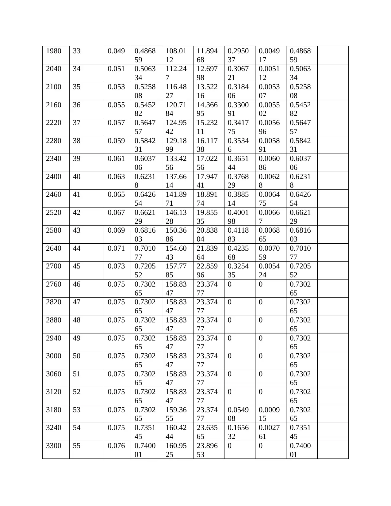
1980 33 0.049 0.4868
59
108.01
12
11.894
68
0.2950
37
0.0049
17
0.4868
59
2040 34 0.051 0.5063
34
112.24
7
12.697
98
0.3067
21
0.0051
12
0.5063
34
2100 35 0.053 0.5258
08
116.48
27
13.522
16
0.3184
06
0.0053
07
0.5258
08
2160 36 0.055 0.5452
82
120.71
84
14.366
95
0.3300
91
0.0055
02
0.5452
82
2220 37 0.057 0.5647
57
124.95
42
15.232
11
0.3417
75
0.0056
96
0.5647
57
2280 38 0.059 0.5842
31
129.18
99
16.117
38
0.3534
6
0.0058
91
0.5842
31
2340 39 0.061 0.6037
06
133.42
56
17.022
56
0.3651
44
0.0060
86
0.6037
06
2400 40 0.063 0.6231
8
137.66
14
17.947
41
0.3768
29
0.0062
8
0.6231
8
2460 41 0.065 0.6426
54
141.89
71
18.891
74
0.3885
14
0.0064
75
0.6426
54
2520 42 0.067 0.6621
29
146.13
28
19.855
35
0.4001
98
0.0066
7
0.6621
29
2580 43 0.069 0.6816
03
150.36
86
20.838
04
0.4118
83
0.0068
65
0.6816
03
2640 44 0.071 0.7010
77
154.60
43
21.839
64
0.4235
68
0.0070
59
0.7010
77
2700 45 0.073 0.7205
52
157.77
85
22.859
96
0.3254
35
0.0054
24
0.7205
52
2760 46 0.075 0.7302
65
158.83
47
23.374
77
0 0 0.7302
65
2820 47 0.075 0.7302
65
158.83
47
23.374
77
0 0 0.7302
65
2880 48 0.075 0.7302
65
158.83
47
23.374
77
0 0 0.7302
65
2940 49 0.075 0.7302
65
158.83
47
23.374
77
0 0 0.7302
65
3000 50 0.075 0.7302
65
158.83
47
23.374
77
0 0 0.7302
65
3060 51 0.075 0.7302
65
158.83
47
23.374
77
0 0 0.7302
65
3120 52 0.075 0.7302
65
158.83
47
23.374
77
0 0 0.7302
65
3180 53 0.075 0.7302
65
159.36
55
23.374
77
0.0549
08
0.0009
15
0.7302
65
3240 54 0.075 0.7351
45
160.42
44
23.635
65
0.1656
32
0.0027
61
0.7351
45
3300 55 0.076 0.7400
01
160.95
25
23.896
53
0 0 0.7400
01
59
108.01
12
11.894
68
0.2950
37
0.0049
17
0.4868
59
2040 34 0.051 0.5063
34
112.24
7
12.697
98
0.3067
21
0.0051
12
0.5063
34
2100 35 0.053 0.5258
08
116.48
27
13.522
16
0.3184
06
0.0053
07
0.5258
08
2160 36 0.055 0.5452
82
120.71
84
14.366
95
0.3300
91
0.0055
02
0.5452
82
2220 37 0.057 0.5647
57
124.95
42
15.232
11
0.3417
75
0.0056
96
0.5647
57
2280 38 0.059 0.5842
31
129.18
99
16.117
38
0.3534
6
0.0058
91
0.5842
31
2340 39 0.061 0.6037
06
133.42
56
17.022
56
0.3651
44
0.0060
86
0.6037
06
2400 40 0.063 0.6231
8
137.66
14
17.947
41
0.3768
29
0.0062
8
0.6231
8
2460 41 0.065 0.6426
54
141.89
71
18.891
74
0.3885
14
0.0064
75
0.6426
54
2520 42 0.067 0.6621
29
146.13
28
19.855
35
0.4001
98
0.0066
7
0.6621
29
2580 43 0.069 0.6816
03
150.36
86
20.838
04
0.4118
83
0.0068
65
0.6816
03
2640 44 0.071 0.7010
77
154.60
43
21.839
64
0.4235
68
0.0070
59
0.7010
77
2700 45 0.073 0.7205
52
157.77
85
22.859
96
0.3254
35
0.0054
24
0.7205
52
2760 46 0.075 0.7302
65
158.83
47
23.374
77
0 0 0.7302
65
2820 47 0.075 0.7302
65
158.83
47
23.374
77
0 0 0.7302
65
2880 48 0.075 0.7302
65
158.83
47
23.374
77
0 0 0.7302
65
2940 49 0.075 0.7302
65
158.83
47
23.374
77
0 0 0.7302
65
3000 50 0.075 0.7302
65
158.83
47
23.374
77
0 0 0.7302
65
3060 51 0.075 0.7302
65
158.83
47
23.374
77
0 0 0.7302
65
3120 52 0.075 0.7302
65
158.83
47
23.374
77
0 0 0.7302
65
3180 53 0.075 0.7302
65
159.36
55
23.374
77
0.0549
08
0.0009
15
0.7302
65
3240 54 0.075 0.7351
45
160.42
44
23.635
65
0.1656
32
0.0027
61
0.7351
45
3300 55 0.076 0.7400
01
160.95
25
23.896
53
0 0 0.7400
01
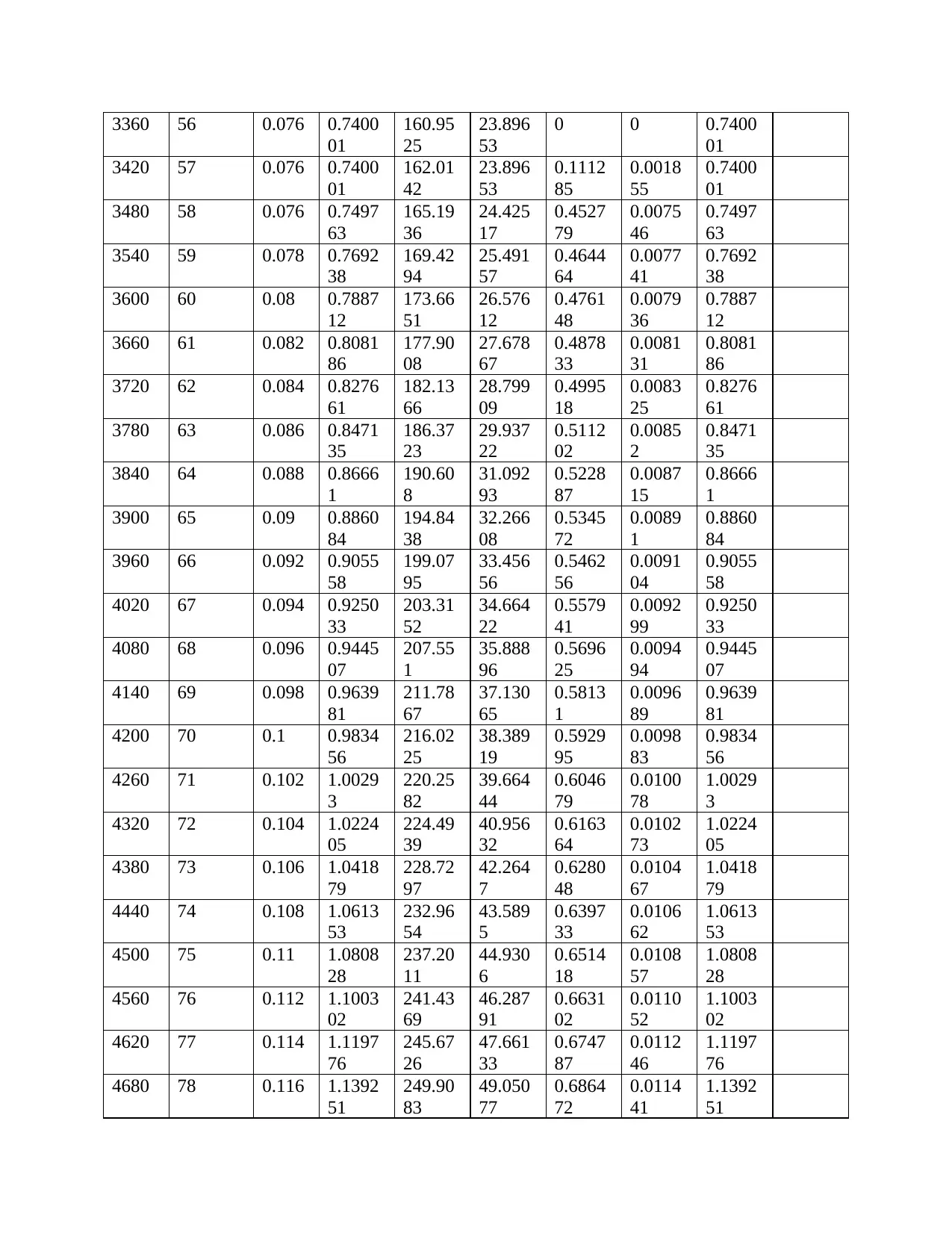
3360 56 0.076 0.7400
01
160.95
25
23.896
53
0 0 0.7400
01
3420 57 0.076 0.7400
01
162.01
42
23.896
53
0.1112
85
0.0018
55
0.7400
01
3480 58 0.076 0.7497
63
165.19
36
24.425
17
0.4527
79
0.0075
46
0.7497
63
3540 59 0.078 0.7692
38
169.42
94
25.491
57
0.4644
64
0.0077
41
0.7692
38
3600 60 0.08 0.7887
12
173.66
51
26.576
12
0.4761
48
0.0079
36
0.7887
12
3660 61 0.082 0.8081
86
177.90
08
27.678
67
0.4878
33
0.0081
31
0.8081
86
3720 62 0.084 0.8276
61
182.13
66
28.799
09
0.4995
18
0.0083
25
0.8276
61
3780 63 0.086 0.8471
35
186.37
23
29.937
22
0.5112
02
0.0085
2
0.8471
35
3840 64 0.088 0.8666
1
190.60
8
31.092
93
0.5228
87
0.0087
15
0.8666
1
3900 65 0.09 0.8860
84
194.84
38
32.266
08
0.5345
72
0.0089
1
0.8860
84
3960 66 0.092 0.9055
58
199.07
95
33.456
56
0.5462
56
0.0091
04
0.9055
58
4020 67 0.094 0.9250
33
203.31
52
34.664
22
0.5579
41
0.0092
99
0.9250
33
4080 68 0.096 0.9445
07
207.55
1
35.888
96
0.5696
25
0.0094
94
0.9445
07
4140 69 0.098 0.9639
81
211.78
67
37.130
65
0.5813
1
0.0096
89
0.9639
81
4200 70 0.1 0.9834
56
216.02
25
38.389
19
0.5929
95
0.0098
83
0.9834
56
4260 71 0.102 1.0029
3
220.25
82
39.664
44
0.6046
79
0.0100
78
1.0029
3
4320 72 0.104 1.0224
05
224.49
39
40.956
32
0.6163
64
0.0102
73
1.0224
05
4380 73 0.106 1.0418
79
228.72
97
42.264
7
0.6280
48
0.0104
67
1.0418
79
4440 74 0.108 1.0613
53
232.96
54
43.589
5
0.6397
33
0.0106
62
1.0613
53
4500 75 0.11 1.0808
28
237.20
11
44.930
6
0.6514
18
0.0108
57
1.0808
28
4560 76 0.112 1.1003
02
241.43
69
46.287
91
0.6631
02
0.0110
52
1.1003
02
4620 77 0.114 1.1197
76
245.67
26
47.661
33
0.6747
87
0.0112
46
1.1197
76
4680 78 0.116 1.1392
51
249.90
83
49.050
77
0.6864
72
0.0114
41
1.1392
51
01
160.95
25
23.896
53
0 0 0.7400
01
3420 57 0.076 0.7400
01
162.01
42
23.896
53
0.1112
85
0.0018
55
0.7400
01
3480 58 0.076 0.7497
63
165.19
36
24.425
17
0.4527
79
0.0075
46
0.7497
63
3540 59 0.078 0.7692
38
169.42
94
25.491
57
0.4644
64
0.0077
41
0.7692
38
3600 60 0.08 0.7887
12
173.66
51
26.576
12
0.4761
48
0.0079
36
0.7887
12
3660 61 0.082 0.8081
86
177.90
08
27.678
67
0.4878
33
0.0081
31
0.8081
86
3720 62 0.084 0.8276
61
182.13
66
28.799
09
0.4995
18
0.0083
25
0.8276
61
3780 63 0.086 0.8471
35
186.37
23
29.937
22
0.5112
02
0.0085
2
0.8471
35
3840 64 0.088 0.8666
1
190.60
8
31.092
93
0.5228
87
0.0087
15
0.8666
1
3900 65 0.09 0.8860
84
194.84
38
32.266
08
0.5345
72
0.0089
1
0.8860
84
3960 66 0.092 0.9055
58
199.07
95
33.456
56
0.5462
56
0.0091
04
0.9055
58
4020 67 0.094 0.9250
33
203.31
52
34.664
22
0.5579
41
0.0092
99
0.9250
33
4080 68 0.096 0.9445
07
207.55
1
35.888
96
0.5696
25
0.0094
94
0.9445
07
4140 69 0.098 0.9639
81
211.78
67
37.130
65
0.5813
1
0.0096
89
0.9639
81
4200 70 0.1 0.9834
56
216.02
25
38.389
19
0.5929
95
0.0098
83
0.9834
56
4260 71 0.102 1.0029
3
220.25
82
39.664
44
0.6046
79
0.0100
78
1.0029
3
4320 72 0.104 1.0224
05
224.49
39
40.956
32
0.6163
64
0.0102
73
1.0224
05
4380 73 0.106 1.0418
79
228.72
97
42.264
7
0.6280
48
0.0104
67
1.0418
79
4440 74 0.108 1.0613
53
232.96
54
43.589
5
0.6397
33
0.0106
62
1.0613
53
4500 75 0.11 1.0808
28
237.20
11
44.930
6
0.6514
18
0.0108
57
1.0808
28
4560 76 0.112 1.1003
02
241.43
69
46.287
91
0.6631
02
0.0110
52
1.1003
02
4620 77 0.114 1.1197
76
245.67
26
47.661
33
0.6747
87
0.0112
46
1.1197
76
4680 78 0.116 1.1392
51
249.90
83
49.050
77
0.6864
72
0.0114
41
1.1392
51
4740 79 0.118 1.1587
25
254.14
41
50.456
13
0.6981
56
0.0116
36
1.1587
25
4800 80 0.12 1.1782 258.37
98
51.877
34
0.7098
41
0.0118
31
1.1782
4860 81 0.122 1.1976
74
262.61
55
53.314
29
0.7215
25
0.0120
25
1.1976
74
4920 82 0.124 1.2171
48
266.85
13
54.766
9
0.7332
1
0.0122
2
1.2171
48
4980 83 0.126 1.2366
23
271.08
7
56.235
09
0.7448
95
0.0124
15
1.2366
23
5040 84 0.128 1.2560
97
275.32
27
57.718
78
0.7565
79
0.0126
1
1.2560
97
5100 85 0.13 1.2755
71
279.55
85
59.217
89
0.7682
64
0.0128
04
1.2755
71
5160 86 0.132 1.2950
46
283.79
42
60.732
33
0.7799
49
0.0129
99
1.2950
46
5220 87 0.134 1.3145
2
288.02
99
62.262
04
0.7916
33
0.0131
94
1.3145
2
5280 88 0.136 1.3339
94
292.26
57
63.806
93
0.8033
18
0.0133
89
1.3339
94
5340 89 0.138 1.3534
69
296.50
14
65.366
93
0.8150
02
0.0135
83
1.3534
69
5400 90 0.14 1.3729
43
300.73
71
66.941
96
0.8266
87
0.0137
78
1.3729
43
5460 91 0.142 1.3924
18
304.97
29
68.531
96
0.8383
72
0.0139
73
1.3924
18
5520 92 0.144 1.4118
92
309.20
86
70.136
86
0.8500
56
0.0141
68
1.4118
92
5580 93 0.146 1.4313
66
313.44
43
71.756
59
0.8617
41
0.0143
62
1.4313
66
5640 94 0.148 1.4508
41
317.68
01
73.391
07
0.8734
26
0.0145
57
1.4508
41
5700 95 0.15 1.4703
15
321.91
58
75.040
25
0.8851
1
0.0147
52
1.4703
15
5760 96 0.152 1.4897
89
326.15
15
76.704
05
0.8967
95
0.0149
47
1.4897
89
5820 97 0.154 1.5092
64
330.38
73
78.382
42
0.9084
79
0.0151
41
1.5092
64
5880 98 0.156 1.5287
38
334.62
3
80.075
29
0.9201
64
0.0153
36
1.5287
38
5940 99 0.158 1.5482
13
338.85
87
81.782
6
0.9318
49
0.0155
31
1.5482
13
6000 100 0.16 1.5676
87
343.09
45
83.504
29
0.9435
33
0.0157
26
1.5676
87
6060 101 0.162 1.5871
61
347.33
02
85.240
3
0.9552
18
0.0159
2
1.5871
61
25
254.14
41
50.456
13
0.6981
56
0.0116
36
1.1587
25
4800 80 0.12 1.1782 258.37
98
51.877
34
0.7098
41
0.0118
31
1.1782
4860 81 0.122 1.1976
74
262.61
55
53.314
29
0.7215
25
0.0120
25
1.1976
74
4920 82 0.124 1.2171
48
266.85
13
54.766
9
0.7332
1
0.0122
2
1.2171
48
4980 83 0.126 1.2366
23
271.08
7
56.235
09
0.7448
95
0.0124
15
1.2366
23
5040 84 0.128 1.2560
97
275.32
27
57.718
78
0.7565
79
0.0126
1
1.2560
97
5100 85 0.13 1.2755
71
279.55
85
59.217
89
0.7682
64
0.0128
04
1.2755
71
5160 86 0.132 1.2950
46
283.79
42
60.732
33
0.7799
49
0.0129
99
1.2950
46
5220 87 0.134 1.3145
2
288.02
99
62.262
04
0.7916
33
0.0131
94
1.3145
2
5280 88 0.136 1.3339
94
292.26
57
63.806
93
0.8033
18
0.0133
89
1.3339
94
5340 89 0.138 1.3534
69
296.50
14
65.366
93
0.8150
02
0.0135
83
1.3534
69
5400 90 0.14 1.3729
43
300.73
71
66.941
96
0.8266
87
0.0137
78
1.3729
43
5460 91 0.142 1.3924
18
304.97
29
68.531
96
0.8383
72
0.0139
73
1.3924
18
5520 92 0.144 1.4118
92
309.20
86
70.136
86
0.8500
56
0.0141
68
1.4118
92
5580 93 0.146 1.4313
66
313.44
43
71.756
59
0.8617
41
0.0143
62
1.4313
66
5640 94 0.148 1.4508
41
317.68
01
73.391
07
0.8734
26
0.0145
57
1.4508
41
5700 95 0.15 1.4703
15
321.91
58
75.040
25
0.8851
1
0.0147
52
1.4703
15
5760 96 0.152 1.4897
89
326.15
15
76.704
05
0.8967
95
0.0149
47
1.4897
89
5820 97 0.154 1.5092
64
330.38
73
78.382
42
0.9084
79
0.0151
41
1.5092
64
5880 98 0.156 1.5287
38
334.62
3
80.075
29
0.9201
64
0.0153
36
1.5287
38
5940 99 0.158 1.5482
13
338.85
87
81.782
6
0.9318
49
0.0155
31
1.5482
13
6000 100 0.16 1.5676
87
343.09
45
83.504
29
0.9435
33
0.0157
26
1.5676
87
6060 101 0.162 1.5871
61
347.33
02
85.240
3
0.9552
18
0.0159
2
1.5871
61
Paraphrase This Document
Need a fresh take? Get an instant paraphrase of this document with our AI Paraphraser
6120 102 0.164 1.6066
36
351.56
59
86.990
57
0.9669
03
0.0161
15
1.6066
36
6180 103 0.166 1.6261
1
355.80
17
88.755
04
0.9785
87
0.0163
1
1.6261
1
6240 104 0.168 1.6455
84
268.96
86
90.533
65
-
20.363
5
-
0.3393
9
1.6455
84
6300 105 0.17 0.8276
56
-
9450.9
2
45.713
24
-
21.105
2
0.0033
5
0.8276
56
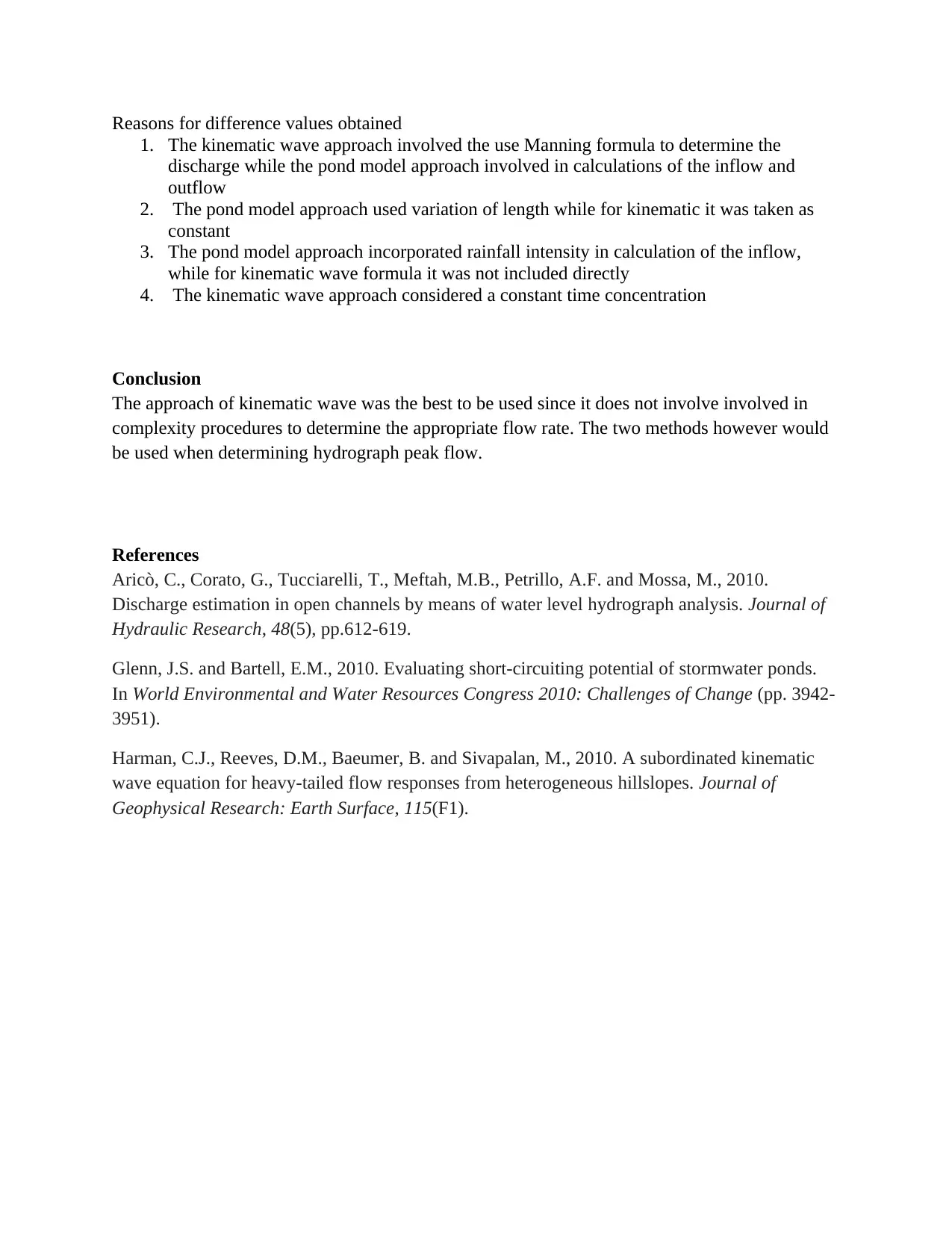
Graphical presentation
0 500 1000 1500 2000 2500 3000 3500
0
0.001
0.002
0.003
0.004
0.005
0.006
0.007
0.008
Flow rate
time in second
flow rate
Comparison of Graph
The report shows the difference between pond model hydrograph and kinematics wave
hydrograph as shown on their respective graphs. The calculated peak discharge for the Kinematic
wave approach was 0.151034 for Pond model approach was 0.007059.
36
351.56
59
86.990
57
0.9669
03
0.0161
15
1.6066
36
6180 103 0.166 1.6261
1
355.80
17
88.755
04
0.9785
87
0.0163
1
1.6261
1
6240 104 0.168 1.6455
84
268.96
86
90.533
65
-
20.363
5
-
0.3393
9
1.6455
84
6300 105 0.17 0.8276
56
-
9450.9
2
45.713
24
-
21.105
2
0.0033
5
0.8276
56
Graphical presentation
0 500 1000 1500 2000 2500 3000 3500
0
0.001
0.002
0.003
0.004
0.005
0.006
0.007
0.008
Flow rate
time in second
flow rate
Comparison of Graph
The report shows the difference between pond model hydrograph and kinematics wave
hydrograph as shown on their respective graphs. The calculated peak discharge for the Kinematic
wave approach was 0.151034 for Pond model approach was 0.007059.
Reasons for difference values obtained
1. The kinematic wave approach involved the use Manning formula to determine the
discharge while the pond model approach involved in calculations of the inflow and
outflow
2. The pond model approach used variation of length while for kinematic it was taken as
constant
3. The pond model approach incorporated rainfall intensity in calculation of the inflow,
while for kinematic wave formula it was not included directly
4. The kinematic wave approach considered a constant time concentration
Conclusion
The approach of kinematic wave was the best to be used since it does not involve involved in
complexity procedures to determine the appropriate flow rate. The two methods however would
be used when determining hydrograph peak flow.
References
Aricò, C., Corato, G., Tucciarelli, T., Meftah, M.B., Petrillo, A.F. and Mossa, M., 2010.
Discharge estimation in open channels by means of water level hydrograph analysis. Journal of
Hydraulic Research, 48(5), pp.612-619.
Glenn, J.S. and Bartell, E.M., 2010. Evaluating short-circuiting potential of stormwater ponds.
In World Environmental and Water Resources Congress 2010: Challenges of Change (pp. 3942-
3951).
Harman, C.J., Reeves, D.M., Baeumer, B. and Sivapalan, M., 2010. A subordinated kinematic
wave equation for heavy‐tailed flow responses from heterogeneous hillslopes. Journal of
Geophysical Research: Earth Surface, 115(F1).
1 out of 15
Your All-in-One AI-Powered Toolkit for Academic Success.
+13062052269
info@desklib.com
Available 24*7 on WhatsApp / Email
![[object Object]](/_next/static/media/star-bottom.7253800d.svg)
Unlock your academic potential
© 2024 | Zucol Services PVT LTD | All rights reserved.