Hypothesis Testing and Probability Analysis Assessment 2022

Running head: STATISTICS 1
Hypothesis Testing and Probability Analysis
Student Name
Professor’s Name
University Name
Date

STATISTICS 2
Hypothesis Testing and Probability Analysis
Assessment Answers by (Insert your name here)
In the summary tables below, insert only the answers. You will show work after the summary
section.
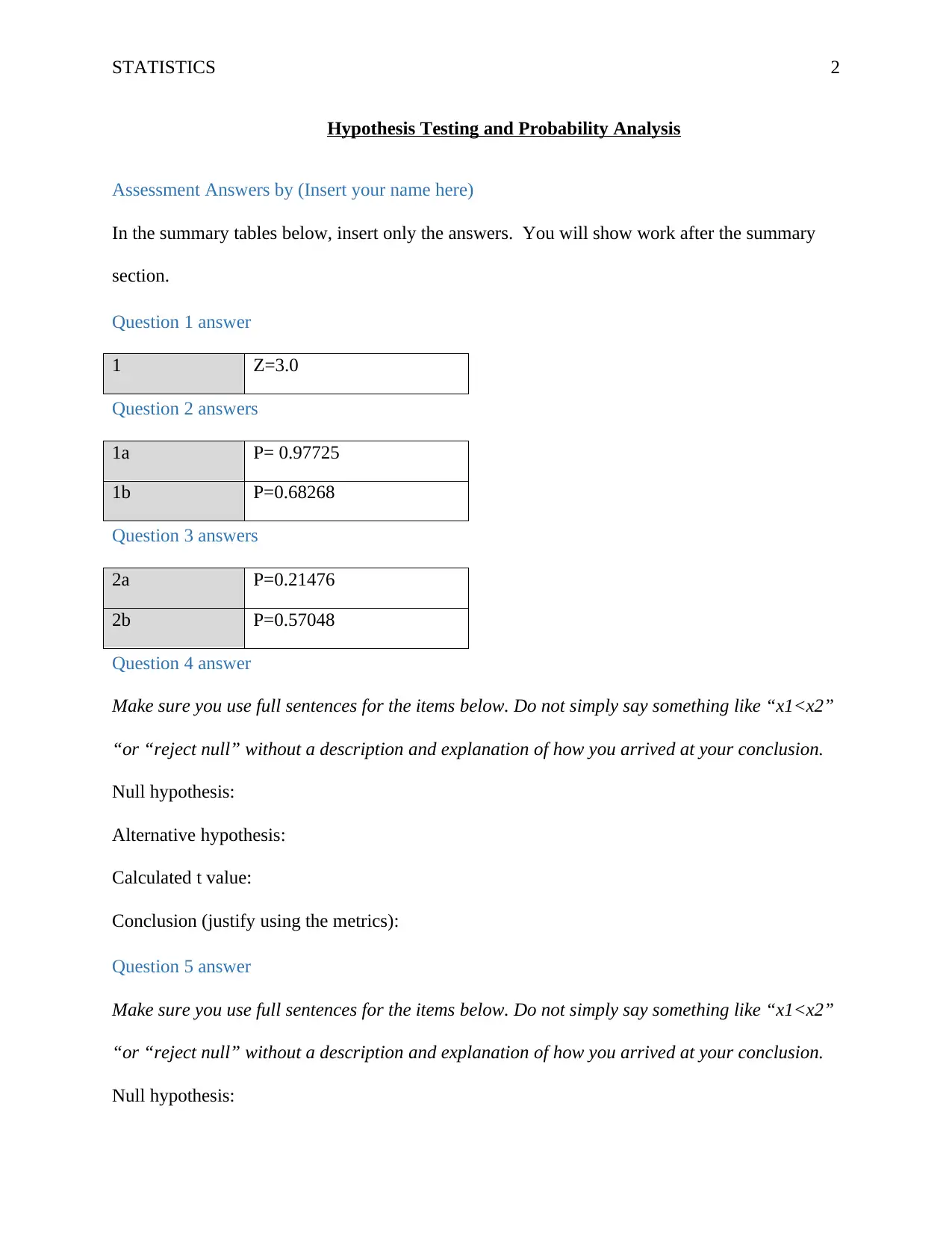
Question 1 answer
1 Z=3.0
Question 2 answers
1a P= 0.97725
1b P=0.68268
Question 3 answers
2a P=0.21476
2b P=0.57048
Question 4 answer
Make sure you use full sentences for the items below. Do not simply say something like “x1<x2”
“or “reject null” without a description and explanation of how you arrived at your conclusion.
Null hypothesis:
Alternative hypothesis:
Calculated t value:
Conclusion (justify using the metrics):
Question 5 answer
Make sure you use full sentences for the items below. Do not simply say something like “x1<x2”
“or “reject null” without a description and explanation of how you arrived at your conclusion.
Null hypothesis:

STATISTICS 3
Alternative hypothesis:
Calculated z value:
Conclusion (justify using the metrics):
Question 6 answer
Make sure you use full sentences for the items below. Do not simply say something like “x1<x2”
“or “reject null” without a description and explanation of how you arrived at your conclusion.
Null hypothesis:
Alternative hypothesis:
Calculated p or t value:
Conclusion (justify using the metrics):
Work
Show all your work for the questions below.
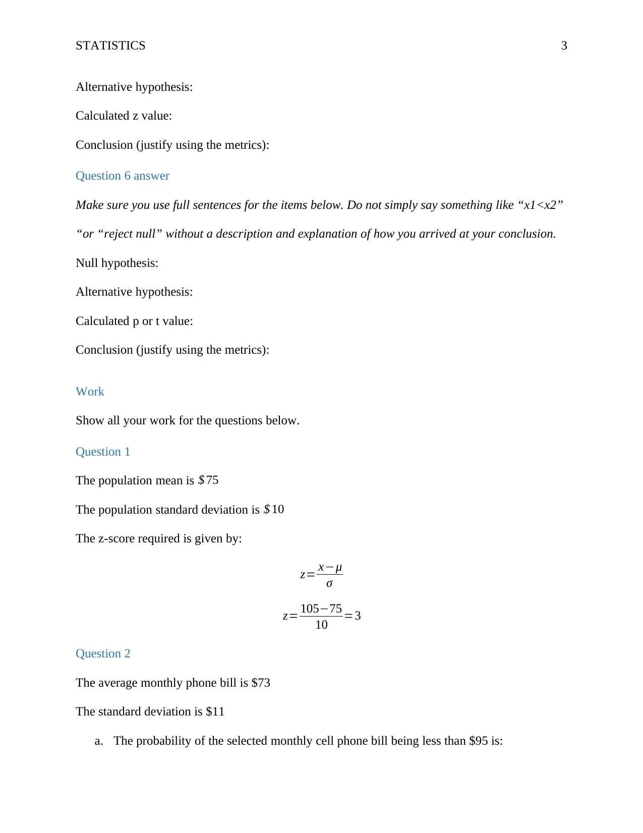
Question 1
The population mean is $ 75
The population standard deviation is $ 10
The z-score required is given by:
z= x−μ
σ
z= 105−75
10 =3
Question 2
The average monthly phone bill is $73
The standard deviation is $11
a. The probability of the selected monthly cell phone bill being less than $95 is:

STATISTICS 4
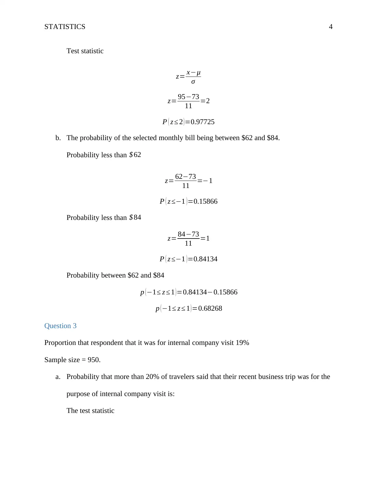
Test statistic
z= x−μ
σ
z= 95−73
11 =2
P ( z ≤ 2 )=0.97725
b. The probability of the selected monthly bill being between $62 and $84.
Probability less than $ 62
z= 62−73
11 =−1
P ( z ≤−1 ) =0.15866
Probability less than $ 84
z= 84−73
11 =1
P ( z ≤−1 ) =0.84134
Probability between $62 and $84
p ( −1≤ z ≤ 1 ) =0.84134−0.15866
p (−1≤ z ≤ 1 )=0.68268
Question 3
Proportion that respondent that it was for internal company visit 19%
Sample size = 950.
a. Probability that more than 20% of travelers said that their recent business trip was for the
purpose of internal company visit is:
The test statistic

STATISTICS 5
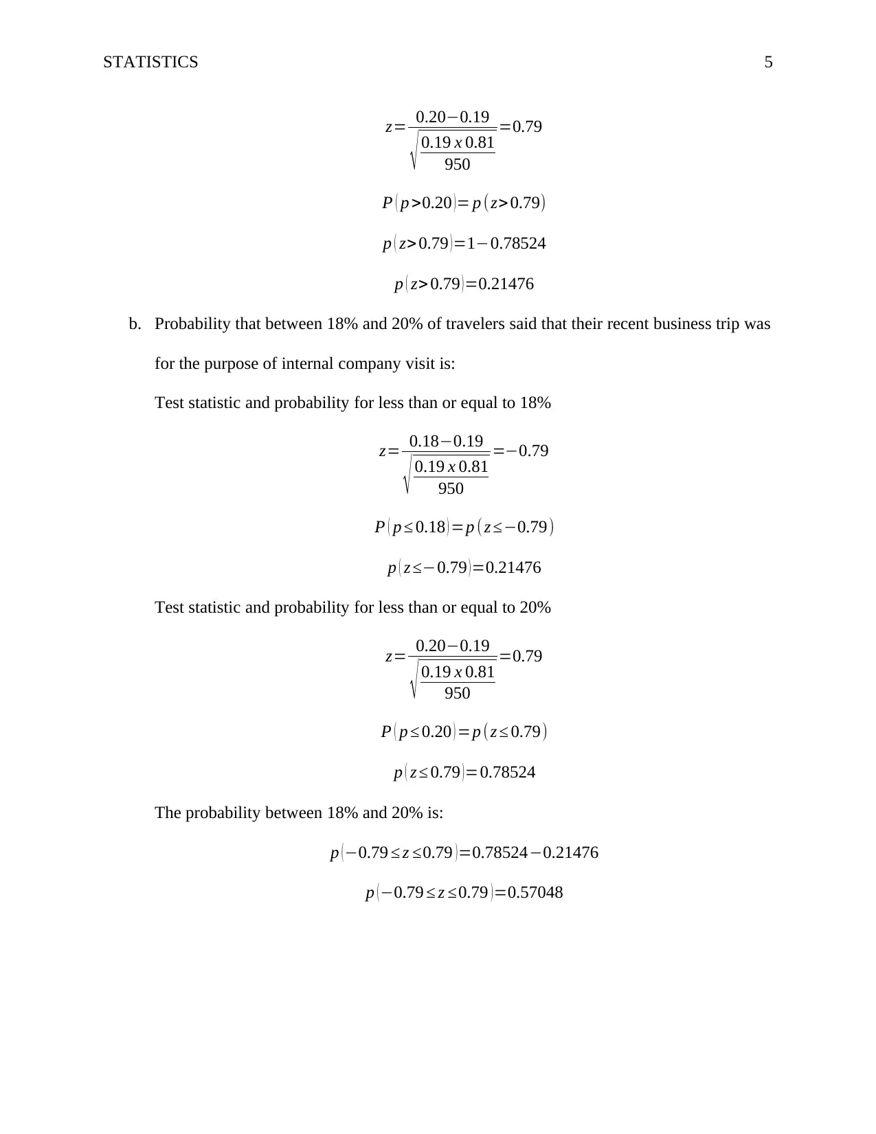
z= 0.20−0.19
√ 0.19 x 0.81
950
=0.79
P ( p >0.20 )= p (z>0.79)
p ( z> 0.79 )=1−0.78524
p ( z> 0.79 )=0.21476
b. Probability that between 18% and 20% of travelers said that their recent business trip was
for the purpose of internal company visit is:
Test statistic and probability for less than or equal to 18%
z= 0.18−0.19
√ 0.19 x 0.81
950
=−0.79
P ( p ≤ 0.18 ) =p ( z ≤−0.79)
p ( z ≤−0.79 )=0.21476
Test statistic and probability for less than or equal to 20%
z= 0.20−0.19
√ 0.19 x 0.81
950
=0.79
P ( p ≤ 0.20 ) =p (z ≤ 0.79)
p ( z ≤ 0.79 )=0.78524
The probability between 18% and 20% is:
p (−0.79 ≤ z ≤0.79 )=0.78524−0.21476
p (−0.79 ≤ z ≤0.79 )=0.57048

STATISTICS 6
Question 4
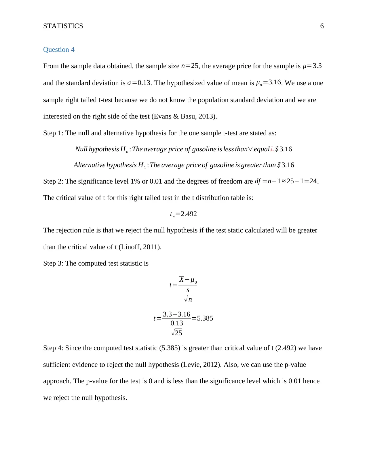
From the sample data obtained, the sample size n=25, the average price for the sample is μ=3.3
and the standard deviation is σ =0.13. The hypothesized value of mean is μo =3.16. We use a one
sample right tailed t-test because we do not know the population standard deviation and we are
interested on the right side of the test (Evans & Basu, 2013).
Step 1: The null and alternative hypothesis for the one sample t-test are stated as:
Null hypothesis Ho : The average price of gasoline is less than∨equal¿ $ 3.16
Alternative hypothesis H1 :The average price of gasoline is greater than $ 3.16
Step 2: The significance level 1% or 0.01 and the degrees of freedom are df =n−1 ≈ 25−1=24.
The critical value of t for this right tailed test in the t distribution table is:
tc=2.492
The rejection rule is that we reject the null hypothesis if the test static calculated will be greater
than the critical value of t (Linoff, 2011).
Step 3: The computed test statistic is
t= X−μ0
s
√n
t= 3.3−3.16
0.13
√25
=5.385
Step 4: Since the computed test statistic (5.385) is greater than critical value of t (2.492) we have
sufficient evidence to reject the null hypothesis (Levie, 2012). Also, we can use the p-value
approach. The p-value for the test is 0 and is less than the significance level which is 0.01 hence
we reject the null hypothesis.

STATISTICS 7
Step 5: The result obtained can be interpreted to mean that since we have rejected the null
hypothesis, we can conveniently conclude that at 0.01 significance level, the average price of
gasoline is greater than $3.16.
Question 5
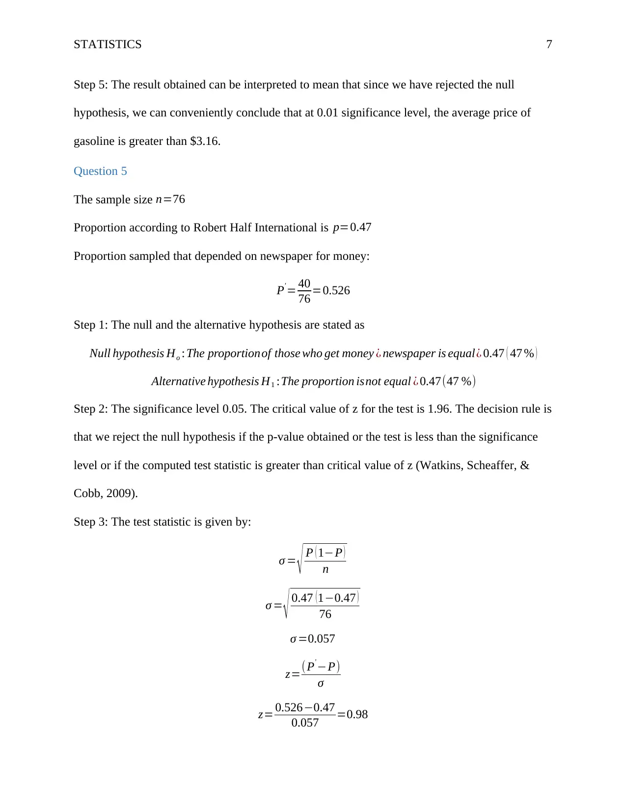
The sample size n=76
Proportion according to Robert Half International is p=0.47
Proportion sampled that depended on newspaper for money:
P' = 40
76 =0.526
Step 1: The null and the alternative hypothesis are stated as
Null hypothesis Ho : The proportionof those who get money ¿ newspaper is equal¿ 0.47 ( 47 % )
Alternative hypothesis H1 :The proportion isnot equal ¿ 0.47(47 %)
Step 2: The significance level 0.05. The critical value of z for the test is 1.96. The decision rule is
that we reject the null hypothesis if the p-value obtained or the test is less than the significance
level or if the computed test statistic is greater than critical value of z (Watkins, Scheaffer, &
Cobb, 2009).
Step 3: The test statistic is given by:
σ = √ P ( 1−P )
n
σ = √ 0.47 (1−0.47 )
76
σ =0.057
z=(P' −P)
σ
z= 0.526−0.47
0.057 =0.98

STATISTICS 8
Step 4: The p-value obtained for the test is 0.8364 and is greater than the significance level
(0.05). Also, the test statistic computed (0.98) is less than the critical value (1.96). Therefore, we
do not reject the null hypothesis.
Step 6: We can interpret the result such that since we do not reject the null hypothesis, there is
sufficient evidence to conclude that the proportion of those who get money from newspaper is
equal to 47% at 0.05 significance level.
Question 6
The null hypothesis and the alternative hypothesis are as stated below:
Null hypothesis Ho : Men∧Women spend the same average amounts on gifts∧cards
Alternative hypothesis Hi : Men∧Women do not spend the same average amounts
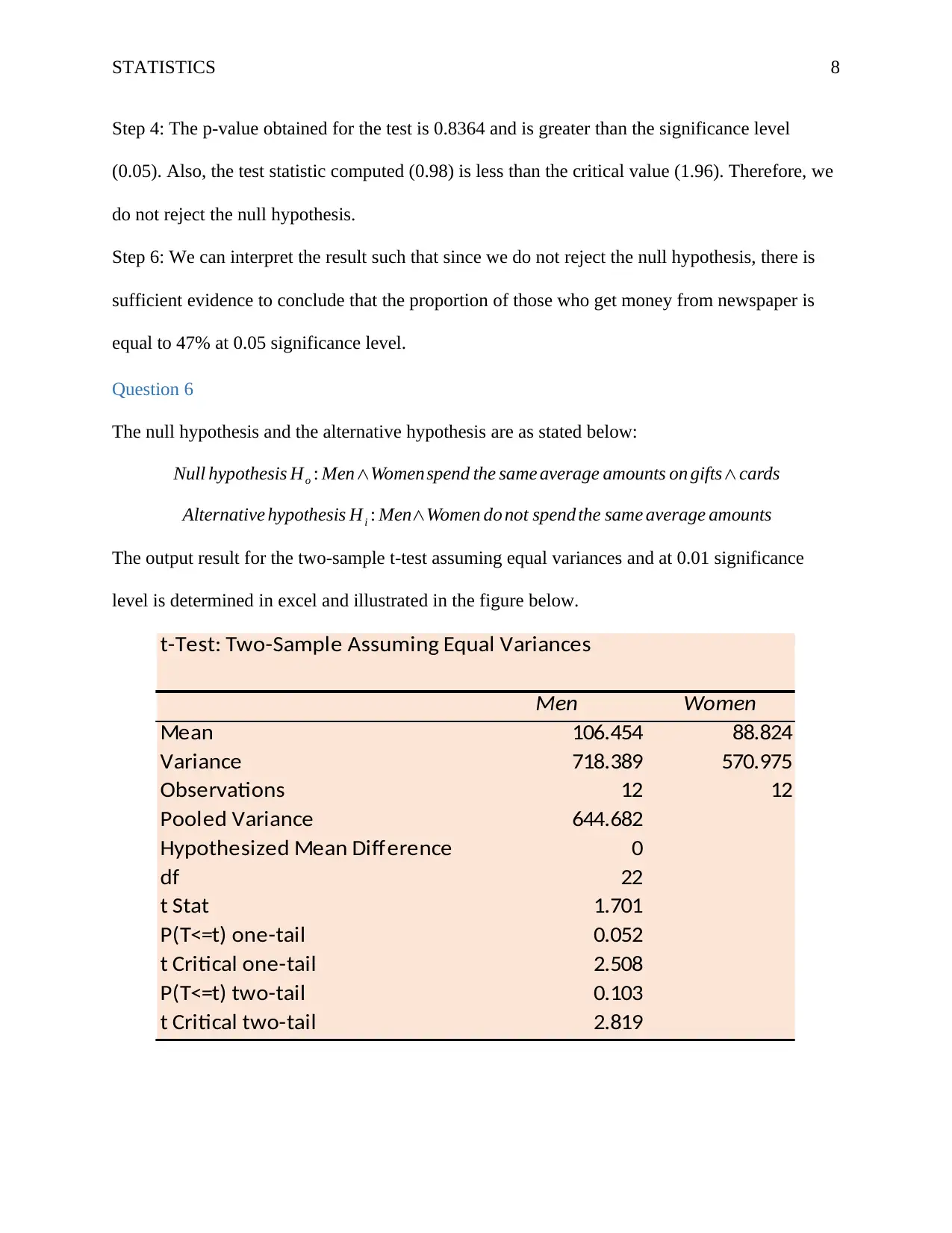
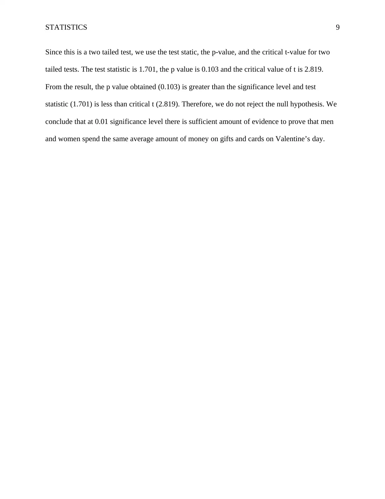
The output result for the two-sample t-test assuming equal variances and at 0.01 significance
level is determined in excel and illustrated in the figure below.
t-Test: Two-Sample Assuming Equal Variances
Men Women
Mean 106.454 88.824
Variance 718.389 570.975
Observations 12 12
Pooled Variance 644.682
Hypothesized Mean Difference 0
df 22
t Stat 1.701
P(T<=t) one-tail 0.052
t Critical one-tail 2.508
P(T<=t) two-tail 0.103
t Critical two-tail 2.819

STATISTICS 9
Since this is a two tailed test, we use the test static, the p-value, and the critical t-value for two
tailed tests. The test statistic is 1.701, the p value is 0.103 and the critical value of t is 2.819.
From the result, the p value obtained (0.103) is greater than the significance level and test
statistic (1.701) is less than critical t (2.819). Therefore, we do not reject the null hypothesis. We
conclude that at 0.01 significance level there is sufficient amount of evidence to prove that men
and women spend the same average amount of money on gifts and cards on Valentine’s day.

STATISTICS 10
References
Evans, J. R., & Basu, A. (2013). Statistics, data analysis, and decision modelling (5th ed).
Boston: Pearson.
Levie, R. D. (2012). Advanced Excel for scientific data analysis (2nd ed). New York, NY: Oxford
University Press.
Linoff, G. (2011). Data analysis using SQL and Excel. Indianapolis, Ind.: Wiley Pub.
Watkins, A. E., Scheaffer, R. L., & Cobb, G. W. (2009). Statistics in action: Understanding a
world of data (2nd ed). Hoboken, NJ: Wiley