Exploration of Ice Cream Data

This essay explores the ice cream data and analyzes the normality of errors in a multiple OLS regression model. It provides insights on the consumption, price, income, and temperature variables. The data is analyzed using descriptive statistics, box plots, and Shapiro-Wilk tests. The results show that income and temperature are significant determinants of ice cream consumption.

Ice Cream Data 1
EXPLORATION OF ICE CREAM DATA
by[Name]
Course
Professor’s Name
Institution
Location of Institution
Date

Ice Cream Data 2
Exploration of Ice Cream Data
Introduction
The dataset was obtained from Kadiyala (1970) article tittle “Testing for
independence of regression disturbance”. The researcher focused on the investigation of
independence of errors in multiple OLS regression model, but the independence assumption
comes after the normality of the residuals are established. The data contained five variables
which were measured on scale, they include the period (weeks), consumption of ice cream
(pints per capita), weekly price (dollar per pint), consumer income (dollars per week) and the
average weekly temperature (0F) (Kadiyala 1970). The sample size was thirty weeks. The
main aim of the essay is to explore the data specifically on the normality of the errors. The
essay begins with a brief introduction of the dataset, followed by description of the data
(Original data and summary statistics). The next section involves discussion of the normality
assumption followed by conclusion.
Description of Ice Cream Data
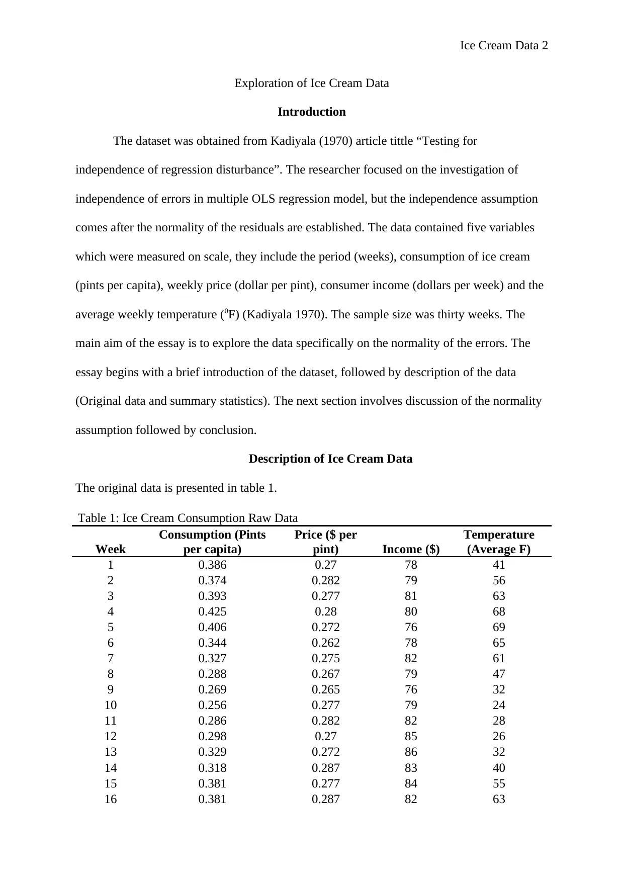
The original data is presented in table 1.
Table 1: Ice Cream Consumption Raw Data
Week
Consumption (Pints
per capita)
Price ($ per
pint) Income ($)
Temperature
(Average F)
1 0.386 0.27 78 41
2 0.374 0.282 79 56
3 0.393 0.277 81 63
4 0.425 0.28 80 68
5 0.406 0.272 76 69
6 0.344 0.262 78 65
7 0.327 0.275 82 61
8 0.288 0.267 79 47
9 0.269 0.265 76 32
10 0.256 0.277 79 24
11 0.286 0.282 82 28
12 0.298 0.27 85 26
13 0.329 0.272 86 32
14 0.318 0.287 83 40
15 0.381 0.277 84 55
16 0.381 0.287 82 63

Ice Cream Data 3
17 0.47 0.28 80 72
18 0.443 0.277 78 72
19 0.386 0.277 84 67
20 0.342 0.277 86 60
21 0.319 0.292 85 44
22 0.307 0.287 87 40
23 0.284 0.277 94 32
24 0.326 0.285 92 27
25 0.309 0.282 95 28
26 0.359 0.265 96 33
27 0.376 0.265 94 41
28 0.416 0.265 96 52
29 0.437 0.268 91 64
30 0.548 0.26 90 71
Source: Kadiyala (1970)
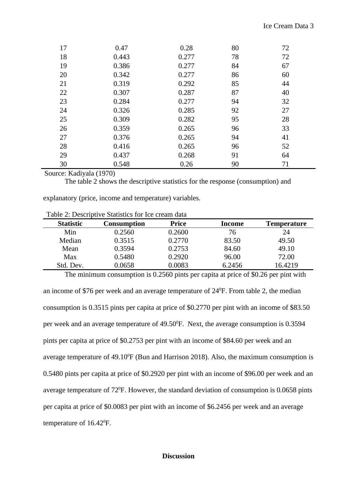
The table 2 shows the descriptive statistics for the response (consumption) and
explanatory (price, income and temperature) variables.
Table 2: Descriptive Statistics for Ice cream data
Statistic Consumption Price Income Temperature
Min 0.2560 0.2600 76 24
Median 0.3515 0.2770 83.50 49.50
Mean 0.3594 0.2753 84.60 49.10
Max 0.5480 0.2920 96.00 72.00
Std. Dev. 0.0658 0.0083 6.2456 16.4219
The minimum consumption is 0.2560 pints per capita at price of $0.26 per pint with
an income of $76 per week and an average temperature of 240F. From table 2, the median
consumption is 0.3515 pints per capita at price of $0.2770 per pint with an income of $83.50
per week and an average temperature of 49.500F. Next, the average consumption is 0.3594
pints per capita at price of $0.2753 per pint with an income of $84.60 per week and an
average temperature of 49.100F (Bun and Harrison 2018). Also, the maximum consumption is
0.5480 pints per capita at price of $0.2920 per pint with an income of $96.00 per week and an
average temperature of 720F. However, the standard deviation of consumption is 0.0658 pints
per capita at price of $0.0083 per pint with an income of $6.2456 per week and an average
temperature of 16.420F.
Discussion

Ice Cream Data 4
The data was mainly collected to test for the behaviour of the residuals that is test the
first assumption of multiple OLS regression (errors are normally distributed with zero mean
and a constant variance). It is of importance to define the contextual meaning of errors, since
the term refer to two concepts relevant to the ordinary least square regression model (Ernst
and Albers 2017). Then, in the context of regression, errors (residuals) are the difference
between actual values of the dependent variable and the predicted values from the regression
estimation for the entire population. It is common knowledge that the errors of a regression
model cannot be directly obtained because the population parameters of the true regression
model are unknown. However, investigation of the characteristics of the errors is possible
through the calculation of residuals of a regression model based on a sample data.
The residuals are the results of the difference between the actual values of the
independent variable and the values forecasted (within sample) by the estimated regression
model. The assumption of errors of regression following an approximate normal distribution
is an important aspect of multiple OLS regression. When the assumption holds, its is possible
to make inferences concerning the regression parameters in the population of origin even if
the sample size is small. The inferences are usually based on confidence intervals or
significance tests (Zhu et al. 2015). An indication that given a small sample size and the
assumption of normality is violated; the inferences will not be trusted since the violation
degrade the efficiency of the estimator. In technical sense, when errors follow a normal
distribution, then OLS is the most efficient among all possible unbiased estimators. But, with
non-normal residuals OLS becomes the most efficient among linear unbiased estimators.
Further, errors that do not follow normal distribution imply that the estimated student
t and F statistics do not follow t and F distributions. Conversely, the assumption of normally
distributed errors is not the only requirement for the estimators of the regression to be
efficient and unbiased. However, for this essay only normality of the errors is considered.

Ice Cream Data 5
Moreover, a larger sample size increases the trustworthiness of the inferences on the
coefficients estimated by the regression model even if the normality assumption is not met
(Doyennette et al 2019). The ice cream data only has 30 sample points therefore, the law of
large numbers will not work. Meaning the assumption must hold for the estimates to be
trustworthy. Multiple OLS regression does not require each variable to be normal distributed
but for this essay normality of the variables are tested using histogram and Shapiro-Wilk test.
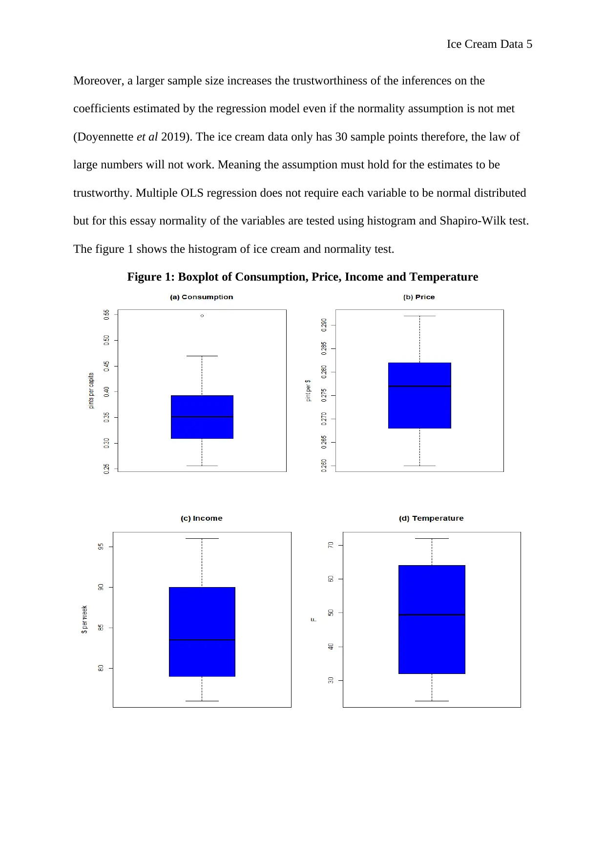
The figure 1 shows the histogram of ice cream and normality test.
Figure 1: Boxplot of Consumption, Price, Income and Temperature

Ice Cream Data 6
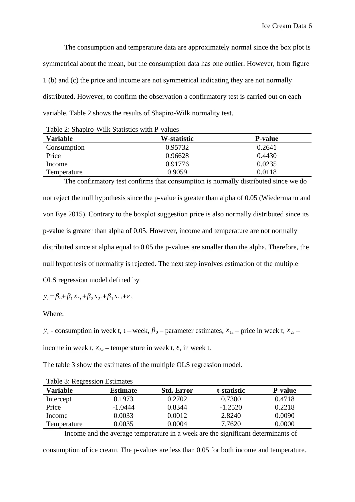
The consumption and temperature data are approximately normal since the box plot is
symmetrical about the mean, but the consumption data has one outlier. However, from figure
1 (b) and (c) the price and income are not symmetrical indicating they are not normally
distributed. However, to confirm the observation a confirmatory test is carried out on each
variable. Table 2 shows the results of Shapiro-Wilk normality test.
Table 2: Shapiro-Wilk Statistics with P-values
Variable W-statistic P-value
Consumption 0.95732 0.2641
Price 0.96628 0.4430
Income 0.91776 0.0235
Temperature 0.9059 0.0118
The confirmatory test confirms that consumption is normally distributed since we do
not reject the null hypothesis since the p-value is greater than alpha of 0.05 (Wiedermann and
von Eye 2015). Contrary to the boxplot suggestion price is also normally distributed since its
p-value is greater than alpha of 0.05. However, income and temperature are not normally
distributed since at alpha equal to 0.05 the p-values are smaller than the alpha. Therefore, the
null hypothesis of normality is rejected. The next step involves estimation of the multiple
OLS regression model defined by
yt =β0+ β1 x1t + β2 x2 t +β1 x1 t +ε t
Where:
yt - consumption in week t, t – week, β0 – parameter estimates, x1 t – price in week t, x2 t –
income in week t, x3 t – temperature in week t, ε t in week t.
The table 3 show the estimates of the multiple OLS regression model.
Table 3: Regression Estimates
Variable Estimate Std. Error t-statistic P-value
Intercept 0.1973 0.2702 0.7300 0.4718
Price -1.0444 0.8344 -1.2520 0.2218
Income 0.0033 0.0012 2.8240 0.0090
Temperature 0.0035 0.0004 7.7620 0.0000
Income and the average temperature in a week are the significant determinants of
consumption of ice cream. The p-values are less than 0.05 for both income and temperature.

Ice Cream Data 7
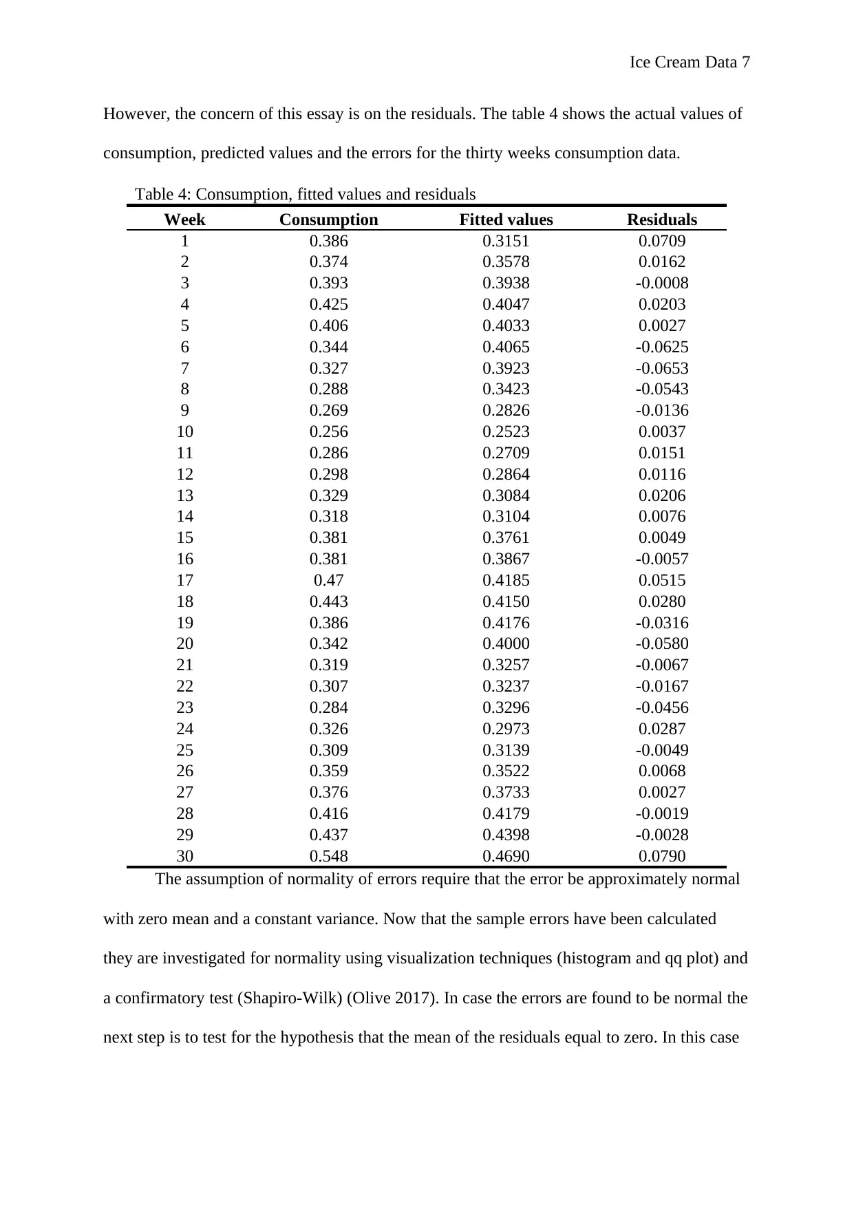
However, the concern of this essay is on the residuals. The table 4 shows the actual values of
consumption, predicted values and the errors for the thirty weeks consumption data.
Table 4: Consumption, fitted values and residuals
Week Consumption Fitted values Residuals
1 0.386 0.3151 0.0709
2 0.374 0.3578 0.0162
3 0.393 0.3938 -0.0008
4 0.425 0.4047 0.0203
5 0.406 0.4033 0.0027
6 0.344 0.4065 -0.0625
7 0.327 0.3923 -0.0653
8 0.288 0.3423 -0.0543
9 0.269 0.2826 -0.0136
10 0.256 0.2523 0.0037
11 0.286 0.2709 0.0151
12 0.298 0.2864 0.0116
13 0.329 0.3084 0.0206
14 0.318 0.3104 0.0076
15 0.381 0.3761 0.0049
16 0.381 0.3867 -0.0057
17 0.47 0.4185 0.0515
18 0.443 0.4150 0.0280
19 0.386 0.4176 -0.0316
20 0.342 0.4000 -0.0580
21 0.319 0.3257 -0.0067
22 0.307 0.3237 -0.0167
23 0.284 0.3296 -0.0456
24 0.326 0.2973 0.0287
25 0.309 0.3139 -0.0049
26 0.359 0.3522 0.0068
27 0.376 0.3733 0.0027
28 0.416 0.4179 -0.0019
29 0.437 0.4398 -0.0028
30 0.548 0.4690 0.0790
The assumption of normality of errors require that the error be approximately normal
with zero mean and a constant variance. Now that the sample errors have been calculated
they are investigated for normality using visualization techniques (histogram and qq plot) and
a confirmatory test (Shapiro-Wilk) (Olive 2017). In case the errors are found to be normal the
next step is to test for the hypothesis that the mean of the residuals equal to zero. In this case

Ice Cream Data 8
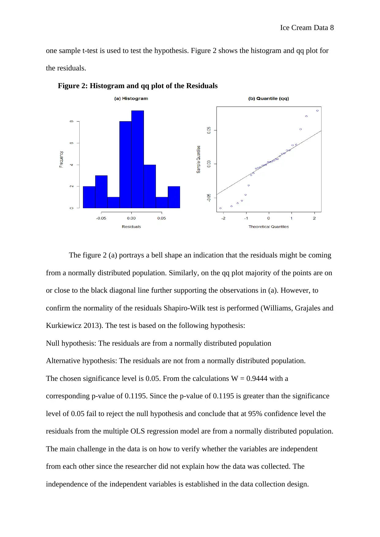
one sample t-test is used to test the hypothesis. Figure 2 shows the histogram and qq plot for
the residuals.
Figure 2: Histogram and qq plot of the Residuals
The figure 2 (a) portrays a bell shape an indication that the residuals might be coming
from a normally distributed population. Similarly, on the qq plot majority of the points are on
or close to the black diagonal line further supporting the observations in (a). However, to
confirm the normality of the residuals Shapiro-Wilk test is performed (Williams, Grajales and
Kurkiewicz 2013). The test is based on the following hypothesis:
Null hypothesis: The residuals are from a normally distributed population
Alternative hypothesis: The residuals are not from a normally distributed population.
The chosen significance level is 0.05. From the calculations W = 0.9444 with a
corresponding p-value of 0.1195. Since the p-value of 0.1195 is greater than the significance
level of 0.05 fail to reject the null hypothesis and conclude that at 95% confidence level the
residuals from the multiple OLS regression model are from a normally distributed population.
The main challenge in the data is on how to verify whether the variables are independent
from each other since the researcher did not explain how the data was collected. The
independence of the independent variables is established in the data collection design.

Ice Cream Data 9
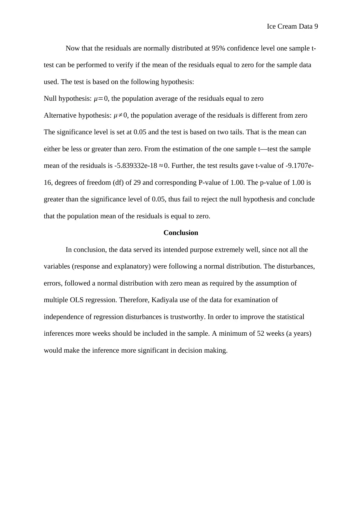
Now that the residuals are normally distributed at 95% confidence level one sample t-
test can be performed to verify if the mean of the residuals equal to zero for the sample data
used. The test is based on the following hypothesis:
Null hypothesis: μ=0, the population average of the residuals equal to zero
Alternative hypothesis: μ ≠ 0, the population average of the residuals is different from zero
The significance level is set at 0.05 and the test is based on two tails. That is the mean can
either be less or greater than zero. From the estimation of the one sample t—test the sample
mean of the residuals is -5.839332e-18 ≈ 0. Further, the test results gave t-value of -9.1707e-
16, degrees of freedom (df) of 29 and corresponding P-value of 1.00. The p-value of 1.00 is
greater than the significance level of 0.05, thus fail to reject the null hypothesis and conclude
that the population mean of the residuals is equal to zero.
Conclusion
In conclusion, the data served its intended purpose extremely well, since not all the
variables (response and explanatory) were following a normal distribution. The disturbances,
errors, followed a normal distribution with zero mean as required by the assumption of
multiple OLS regression. Therefore, Kadiyala use of the data for examination of
independence of regression disturbances is trustworthy. In order to improve the statistical
inferences more weeks should be included in the sample. A minimum of 52 weeks (a years)
would make the inference more significant in decision making.

Ice Cream Data 10
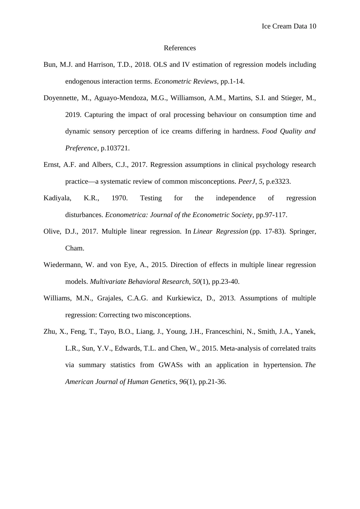
References
Bun, M.J. and Harrison, T.D., 2018. OLS and IV estimation of regression models including
endogenous interaction terms. Econometric Reviews, pp.1-14.
Doyennette, M., Aguayo-Mendoza, M.G., Williamson, A.M., Martins, S.I. and Stieger, M.,
2019. Capturing the impact of oral processing behaviour on consumption time and
dynamic sensory perception of ice creams differing in hardness. Food Quality and
Preference, p.103721.
Ernst, A.F. and Albers, C.J., 2017. Regression assumptions in clinical psychology research
practice—a systematic review of common misconceptions. PeerJ, 5, p.e3323.
Kadiyala, K.R., 1970. Testing for the independence of regression
disturbances. Econometrica: Journal of the Econometric Society, pp.97-117.
Olive, D.J., 2017. Multiple linear regression. In Linear Regression (pp. 17-83). Springer,
Cham.
Wiedermann, W. and von Eye, A., 2015. Direction of effects in multiple linear regression
models. Multivariate Behavioral Research, 50(1), pp.23-40.
Williams, M.N., Grajales, C.A.G. and Kurkiewicz, D., 2013. Assumptions of multiple
regression: Correcting two misconceptions.
Zhu, X., Feng, T., Tayo, B.O., Liang, J., Young, J.H., Franceschini, N., Smith, J.A., Yanek,
L.R., Sun, Y.V., Edwards, T.L. and Chen, W., 2015. Meta-analysis of correlated traits
via summary statistics from GWASs with an application in hypertension. The
American Journal of Human Genetics, 96(1), pp.21-36.

Ice Cream Data 11
Appendix
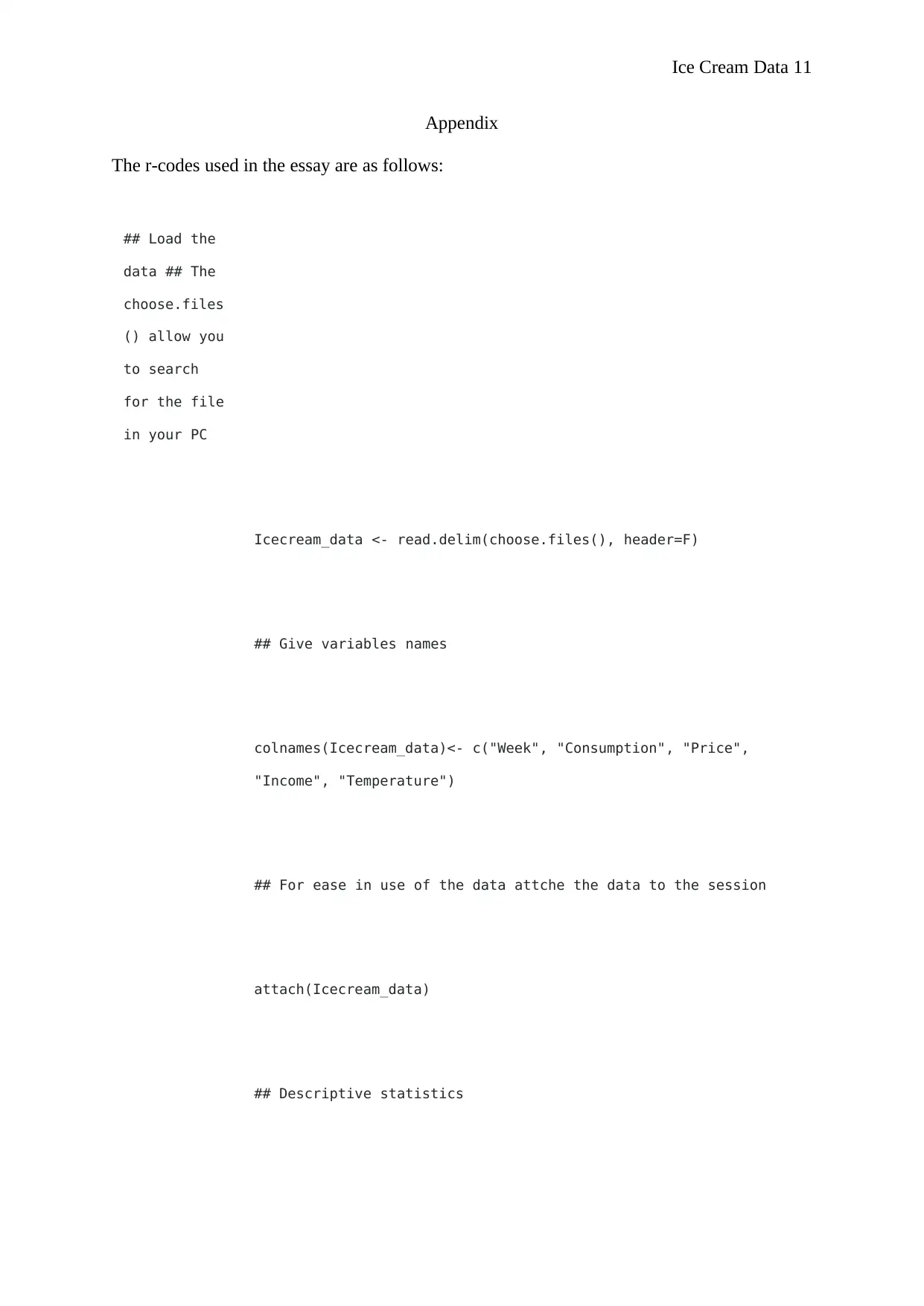
The r-codes used in the essay are as follows:
## Load the
data ## The
choose.files
() allow you
to search
for the file
in your PC
Icecream_data <- read.delim(choose.files(), header=F)
## Give variables names
colnames(Icecream_data)<- c("Week", "Consumption", "Price",
"Income", "Temperature")
## For ease in use of the data attche the data to the session
attach(Icecream_data)
## Descriptive statistics

Ice Cream Data 12
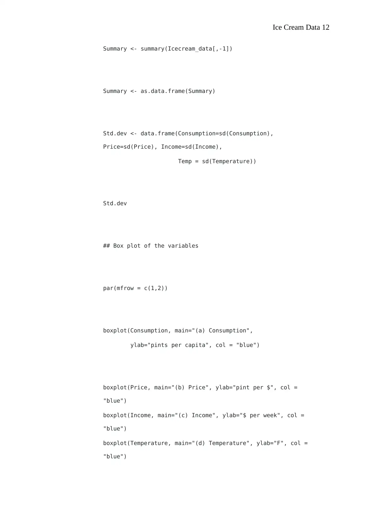
Summary <- summary(Icecream_data[,-1])
Summary <- as.data.frame(Summary)
Std.dev <- data.frame(Consumption=sd(Consumption),
Price=sd(Price), Income=sd(Income),
Temp = sd(Temperature))
Std.dev
## Box plot of the variables
par(mfrow = c(1,2))
boxplot(Consumption, main="(a) Consumption",
ylab="pints per capita", col = "blue")
boxplot(Price, main="(b) Price", ylab="pint per $", col =
"blue")
boxplot(Income, main="(c) Income", ylab="$ per week", col =
"blue")
boxplot(Temperature, main="(d) Temperature", ylab="F", col =
"blue")

Ice Cream Data 13
## Normalit test
T1 <- shapiro.test(Consumption)
T2 <- shapiro.test(Price)
T3 <- shapiro.test(Income)
T4 <- shapiro.test(Temperature)
## Results
T1;T2;T3;T4
### Regression estimation
Mod <- lm(Consumption~Price+Income+Temperature)
summary(Mod)
## Fitted values
fitted_values <- Mod$fitted.values
fitted_values <- as.data.frame(fitted_values)

Ice Cream Data 14
## Combine it with the week and consumption data
New_data <- cbind(Icecream_data[, c(1,2)], fitted_values)
### Residuals
Residuals <-Mod$residuals
Residuals <- as.data.frame(Residuals)
## Make the final dataset
New_data <- cbind(New_data, Residuals)
attach(New_data)
## Histogram and qqplot for residuals
hist(New_data$Residuals, main = "(a) Histogram", ylab =
"Frequency",xlab = "Residuals",
col = "blue")
qqnorm(New_data$Residuals, main = "(b) Quantile (qq)",

Ice Cream Data 15
col="blue")
qqline(New_data$Residuals, col="black")
## Normality test for residuals
shapiro.test(New_data$Residuals)
## Hypothesis testing (one-sample t-test)
t.test(New_data$Residuals, mu=0, alternative = "two.sided")