Application of Multiple Linear Regression Model and Data Changes

II. Application of the model and the data
A. Database Changes
In order to perform multiple linear regression, there are preliminary steps such as
coding of the categorical and ordinal variables: The annex 2 in the annex shows the coding
used for the variables. The table 1 shows the descriptive statistics for the scale variables.
Table 1: Descriptive Statistic for the Scale Variables
Statistic Type (No. of Rooms) Price (Euros) Area (Square meters)
Mean 3.09 922768.50 78.919
Std. Deviation 1.569 695562.284 58.9987
Range 8 2838000 255.5
Minimum 1 222000 23.0
Maximum 9 3060000 278.5
Valid 54 54 54
Source: Author (2019)
On average a house with three rooms and an area of 78.919 square meters sells for an
average of 922,769 Euros in Paris. Further, the minimum number of rooms available for a
house inn Paris is one while the maximum is nine. The maximum price for nine roomed
house averages at 3,060,000 Euros. The maximum area available is 278.5 squared meters
while the minimum for one roomed house is 23 squared meters. Additionally, the descriptive
statistics for categorical variables are shown in annex.
The data contain twelve independent variables and one independent variables. Given
the large number of variables forward selection procedure was performed to select the
significant variables and include in the regression model. The regression model is of the
form:
Y i=β1 X1 + β2 X2 + β3 X3 + β4 X4 + β5 X5 + β6 X6 + β7 X7+ β8 X8 + β9 X9 + β10 X10+ β11 X11+ εi
Where:
Y i – Price of the house in Euros
βi
' s – Parameter estimates i = 1, 2..., 12.

Xi – are the predictor variables.
Presented in the annex are the outputs of the regression analysis. From the model
summary the R-squared = 95.09% indicating that 95% of the variations in price on average
are explained by the independent variables included in the model. This is a good indication
that the model fits the data correctly. Further, the F-statistic = 66.23 with corresponding p-
value = 0.000 indicating that the overall model is fit and hence appropriate for prediction of
the price of a house in Paris.
The constant term is not included in the model since it does not any economical
meaning because we cannot have a house with zero number of rooms, area, district,
luminosity. The p-value for type (number of rooms) is 0.023 indicating that the number of
rooms is important in determining the price of the house in Paris. The area (square meters) is
also having small p-value = 0.000 indicating that it is significant in determining the price of a
house in Paris. Moreover, a house located in district 5, 10, 13, 15, 17 and 18 have p-values
above 0.05 indicating that these locations do not affect the price of a house in Paris. While
locating a house in district 4 and 12 significantly determines the price of the house in Paris
since the p-values are less than 0.05.
The high p-values for the six districts should be explained by the VIF but that’s not
the case since all the VIF’s are less than 5 hence multi-collinearity does not exist between
these variables. However, for type (number of rooms) and area (square meters) have VIF =
16.17 and 14.32 respectively. These high values show that there exists a co-linearity between
the variables.
B. Multiple Linear Regression model
The analysis was not possible in excel since there variables are mixed between
categorical and scaled measures. Therefore, for this regression Minitab which is closely
related to excel was used in the analysis. The full outputs are presented in the annex section.

However, the most important statistics are presented in the body section. The multiple
regression equation estimated is of the form:
^Y i=β1 X1 + β2 X2 + β3 X3 + β4 X4 + β5 X5
Where:
^Y i – Price in Euros
β1 = 75274, β2 = 8984, β3 = 186203 and β4 = -332005.
X1 – Type (Number of rooms)
X2 – Area (Square meters)
X3 – District 4
X 4 – District 12.
Therefore, the multiple linear regression model is as follows:
Price=75274 Type+ 8984 Square meters+186203 District 4−332005 District 12
The coefficient for Type (number of rooms) is 75274 implying that expansion of a
house to include one more room result in increase of the average price by 75274 euros. The
coefficient for area (square meters) is 8984 implying that one-unit expansion of the area that
a house covers (expanding the house area) by one square meter results on an average increase
in the price of a house by 8984 euros. Also, the parameter estimate is 186203 indicating that a
house located in any part of district 4 improves the average sale price of the house by 186203
euros. Finally, the estimated coefficient for district 12 is -332005 indicating that a house
located in district 12 on average will attract a price less than the market average by 332005
euros. Given the high value of adjusted R2 = 96.94% indicate that the model is fit for the data.
However, the model will be appropriate only if the assumptions of ordinary linear regressions
are met. The assumptions include linearity, independence, normality, and equal variance.
These assumptions are checked using residual analysis and other diagnostic tests.

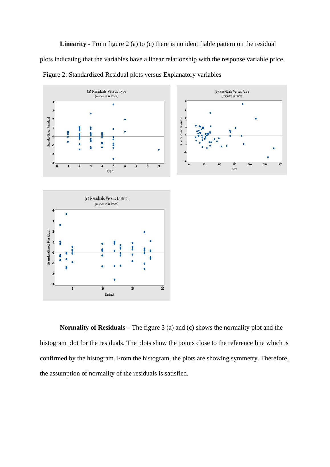
Linearity - From figure 2 (a) to (c) there is no identifiable pattern on the residual
plots indicating that the variables have a linear relationship with the response variable price.
Figure 2: Standardized Residual plots versus Explanatory variables
9876543210
4
3
2
1
0
-1
-2
-3
Type
Standardized Residual
(a) Residuals Versus Type
(response is Price)
300250200150100500
4
3
2
1
0
-1
-2
-3
Area
Standardized Residual
(b) Residuals Versus Area
(response is Price)
2015105
4
3
2
1
0
-1
-2
-3
District
Standardized Residual
(c) Residuals Versus District
(response is Price)
Normality of Residuals – The figure 3 (a) and (c) shows the normality plot and the
histogram plot for the residuals. The plots show the points close to the reference line which is
confirmed by the histogram. From the histogram, the plots are showing symmetry. Therefore,
the assumption of normality of the residuals is satisfied.