Individual Data Analysis Project: UK Schizophrenia Prescriptions
VerifiedAdded on 2022/08/16
|32
|7835
|13
Project
AI Summary
This individual data analysis project investigates the factors influencing the rates of prescriptions for schizophrenia and related psychosis in the United Kingdom. The study utilizes data from 2010/11 and 2015/16, examining the impact of variables such as region, gender, age groups, and population. Employing methodologies including correlation analysis, cluster analysis, Mann Whitney U Test, spatial analysis, and multiple linear regression, the project aims to determine if these variables significantly affect prescription rates. The results indicate that the studied demographic and regional factors do not have a significant impact on the rates of prescriptions. The project also explores the possibility of predicting prescription rates, contributing to a better understanding of the distribution of prescriptions and informing planning for this vulnerable population group. The analysis includes data preparation, descriptive statistics, and inferential analysis, providing a comprehensive overview of the trends and patterns in schizophrenia prescriptions across the UK.
Individual Data Analysis Project
Paraphrase This Document
Need a fresh take? Get an instant paraphrase of this document with our AI Paraphraser
Individual Data Analysis Project
Abstract
The purpose of this study is to determine whether other variables can be used to explain
the difference in rates of prescriptions of schizophrenia and other related psychosis in the United
Kingdom. Data on the rates of prescriptions for 2 periods: 2010/11 and 2015/16 and
demographics are considered for the study. Correlation Analysis and Cluster Analysis are
applied to determine the effect of other variables on the rates of prescriptions. Mann Whitney U
Test and Spatial Analysis are applied to compare the rates of the prescriptions in 2 periods. The
study also looks at the possibility of predicting the rates of prescriptions using multiple linear
regression analysis. The region, proportion of gender, proportion of age groups and population
do not have any significant effect on rates of prescriptions of schizophrenia and other related
psychosis in the United Kingdom.
2
Individual Data Analysis Project
Contents
Introduction.................................................................................................................................................4
Data.............................................................................................................................................................4
Methodology...............................................................................................................................................6
Analysis Results..........................................................................................................................................7
Data Preparation......................................................................................................................................7
Descriptive Analysis..............................................................................................................................11
Inferential Analysis...............................................................................................................................12
Spatial Analysis.................................................................................................................................12
Correlation Analysis..........................................................................................................................13
Cluster Analysis.................................................................................................................................15
Independent Sample T-test................................................................................................................18
Mann Whitney U Test.......................................................................................................................19
Prediction Analysis............................................................................................................................20
Conclusion.................................................................................................................................................21
References.................................................................................................................................................22
Appendix: R Script....................................................................................................................................24
3
⊘ This is a preview!⊘
Do you want full access?
Subscribe today to unlock all pages.
Trusted by 1+ million students worldwide
Individual Data Analysis Project
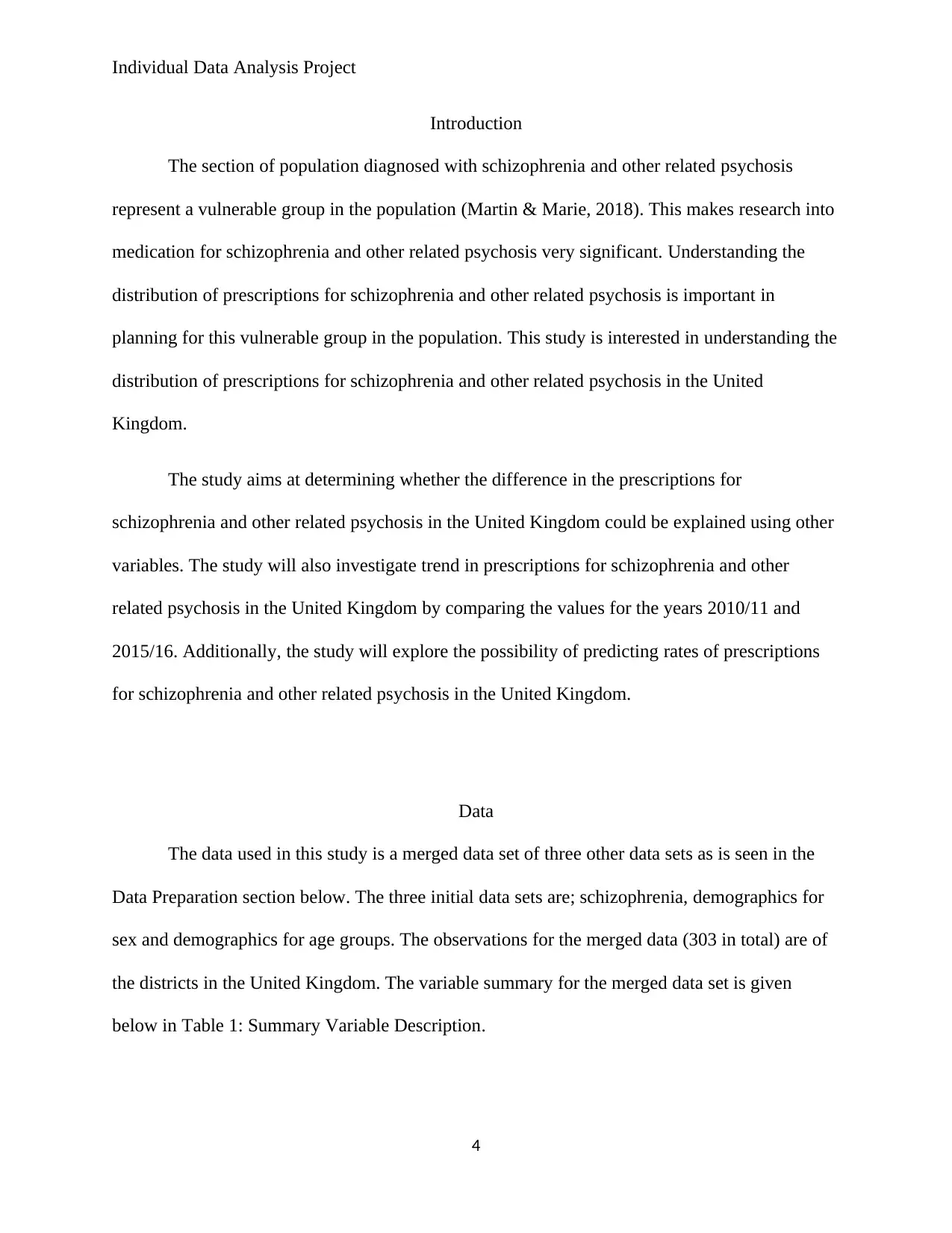
Introduction
The section of population diagnosed with schizophrenia and other related psychosis
represent a vulnerable group in the population (Martin & Marie, 2018). This makes research into
medication for schizophrenia and other related psychosis very significant. Understanding the
distribution of prescriptions for schizophrenia and other related psychosis is important in
planning for this vulnerable group in the population. This study is interested in understanding the
distribution of prescriptions for schizophrenia and other related psychosis in the United
Kingdom.
The study aims at determining whether the difference in the prescriptions for
schizophrenia and other related psychosis in the United Kingdom could be explained using other
variables. The study will also investigate trend in prescriptions for schizophrenia and other
related psychosis in the United Kingdom by comparing the values for the years 2010/11 and
2015/16. Additionally, the study will explore the possibility of predicting rates of prescriptions
for schizophrenia and other related psychosis in the United Kingdom.
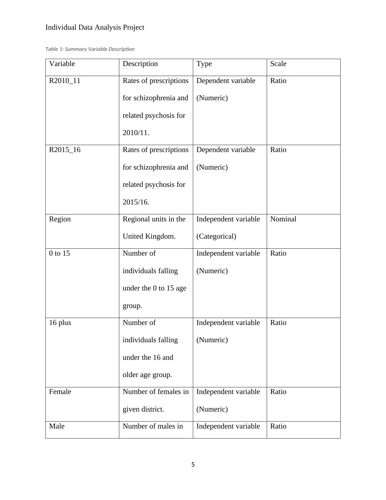
Data
The data used in this study is a merged data set of three other data sets as is seen in the
Data Preparation section below. The three initial data sets are; schizophrenia, demographics for
sex and demographics for age groups. The observations for the merged data (303 in total) are of
the districts in the United Kingdom. The variable summary for the merged data set is given
below in Table 1: Summary Variable Description.
4
Introduction
The section of population diagnosed with schizophrenia and other related psychosis
represent a vulnerable group in the population (Martin & Marie, 2018). This makes research into
medication for schizophrenia and other related psychosis very significant. Understanding the
distribution of prescriptions for schizophrenia and other related psychosis is important in
planning for this vulnerable group in the population. This study is interested in understanding the
distribution of prescriptions for schizophrenia and other related psychosis in the United
Kingdom.
The study aims at determining whether the difference in the prescriptions for
schizophrenia and other related psychosis in the United Kingdom could be explained using other
variables. The study will also investigate trend in prescriptions for schizophrenia and other
related psychosis in the United Kingdom by comparing the values for the years 2010/11 and
2015/16. Additionally, the study will explore the possibility of predicting rates of prescriptions
for schizophrenia and other related psychosis in the United Kingdom.
Data
The data used in this study is a merged data set of three other data sets as is seen in the
Data Preparation section below. The three initial data sets are; schizophrenia, demographics for
sex and demographics for age groups. The observations for the merged data (303 in total) are of
the districts in the United Kingdom. The variable summary for the merged data set is given
below in Table 1: Summary Variable Description.
4
Paraphrase This Document
Need a fresh take? Get an instant paraphrase of this document with our AI Paraphraser
Individual Data Analysis Project
Table 1: Summary Variable Description
Variable Description Type Scale
R2010_11 Rates of prescriptions
for schizophrenia and
related psychosis for
2010/11.
Dependent variable
(Numeric)
Ratio
R2015_16 Rates of prescriptions
for schizophrenia and
related psychosis for
2015/16.
Dependent variable
(Numeric)
Ratio
Region Regional units in the
United Kingdom.
Independent variable
(Categorical)
Nominal
0 to 15 Number of
individuals falling
under the 0 to 15 age
group.
Independent variable
(Numeric)
Ratio
16 plus Number of
individuals falling
under the 16 and
older age group.
Independent variable
(Numeric)
Ratio
Female Number of females in
given district.
Independent variable
(Numeric)
Ratio
Male Number of males in Independent variable Ratio
5
Individual Data Analysis Project
given district. (Numeric)
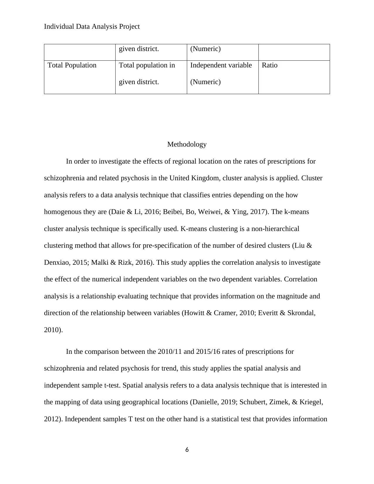
Total Population Total population in
given district.
Independent variable
(Numeric)
Ratio
Methodology
In order to investigate the effects of regional location on the rates of prescriptions for
schizophrenia and related psychosis in the United Kingdom, cluster analysis is applied. Cluster
analysis refers to a data analysis technique that classifies entries depending on the how
homogenous they are (Daie & Li, 2016; Beibei, Bo, Weiwei, & Ying, 2017). The k-means
cluster analysis technique is specifically used. K-means clustering is a non-hierarchical
clustering method that allows for pre-specification of the number of desired clusters (Liu &
Denxiao, 2015; Malki & Rizk, 2016). This study applies the correlation analysis to investigate
the effect of the numerical independent variables on the two dependent variables. Correlation
analysis is a relationship evaluating technique that provides information on the magnitude and
direction of the relationship between variables (Howitt & Cramer, 2010; Everitt & Skrondal,
2010).
In the comparison between the 2010/11 and 2015/16 rates of prescriptions for
schizophrenia and related psychosis for trend, this study applies the spatial analysis and
independent sample t-test. Spatial analysis refers to a data analysis technique that is interested in
the mapping of data using geographical locations (Danielle, 2019; Schubert, Zimek, & Kriegel,
2012). Independent samples T test on the other hand is a statistical test that provides information
6
given district. (Numeric)
Total Population Total population in
given district.
Independent variable
(Numeric)
Ratio
Methodology
In order to investigate the effects of regional location on the rates of prescriptions for
schizophrenia and related psychosis in the United Kingdom, cluster analysis is applied. Cluster
analysis refers to a data analysis technique that classifies entries depending on the how
homogenous they are (Daie & Li, 2016; Beibei, Bo, Weiwei, & Ying, 2017). The k-means
cluster analysis technique is specifically used. K-means clustering is a non-hierarchical
clustering method that allows for pre-specification of the number of desired clusters (Liu &
Denxiao, 2015; Malki & Rizk, 2016). This study applies the correlation analysis to investigate
the effect of the numerical independent variables on the two dependent variables. Correlation
analysis is a relationship evaluating technique that provides information on the magnitude and
direction of the relationship between variables (Howitt & Cramer, 2010; Everitt & Skrondal,
2010).
In the comparison between the 2010/11 and 2015/16 rates of prescriptions for
schizophrenia and related psychosis for trend, this study applies the spatial analysis and
independent sample t-test. Spatial analysis refers to a data analysis technique that is interested in
the mapping of data using geographical locations (Danielle, 2019; Schubert, Zimek, & Kriegel,
2012). Independent samples T test on the other hand is a statistical test that provides information
6
⊘ This is a preview!⊘
Do you want full access?
Subscribe today to unlock all pages.
Trusted by 1+ million students worldwide
Individual Data Analysis Project
on whether two populations that are independent of each other are statistically different (Barbara
& Susan, 2014; Keller, 2015).
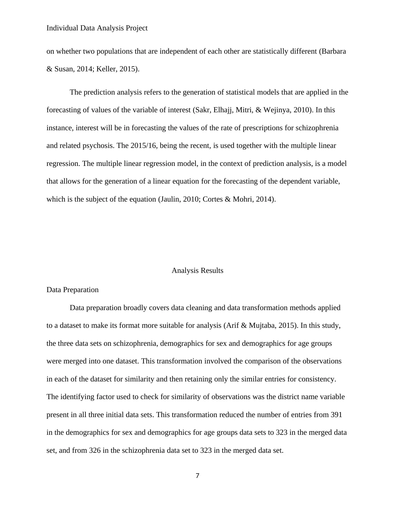
The prediction analysis refers to the generation of statistical models that are applied in the
forecasting of values of the variable of interest (Sakr, Elhajj, Mitri, & Wejinya, 2010). In this
instance, interest will be in forecasting the values of the rate of prescriptions for schizophrenia
and related psychosis. The 2015/16, being the recent, is used together with the multiple linear
regression. The multiple linear regression model, in the context of prediction analysis, is a model
that allows for the generation of a linear equation for the forecasting of the dependent variable,
which is the subject of the equation (Jaulin, 2010; Cortes & Mohri, 2014).
Analysis Results
Data Preparation
Data preparation broadly covers data cleaning and data transformation methods applied
to a dataset to make its format more suitable for analysis (Arif & Mujtaba, 2015). In this study,
the three data sets on schizophrenia, demographics for sex and demographics for age groups
were merged into one dataset. This transformation involved the comparison of the observations
in each of the dataset for similarity and then retaining only the similar entries for consistency.
The identifying factor used to check for similarity of observations was the district name variable
present in all three initial data sets. This transformation reduced the number of entries from 391
in the demographics for sex and demographics for age groups data sets to 323 in the merged data
set, and from 326 in the schizophrenia data set to 323 in the merged data set.
7
on whether two populations that are independent of each other are statistically different (Barbara
& Susan, 2014; Keller, 2015).
The prediction analysis refers to the generation of statistical models that are applied in the
forecasting of values of the variable of interest (Sakr, Elhajj, Mitri, & Wejinya, 2010). In this
instance, interest will be in forecasting the values of the rate of prescriptions for schizophrenia
and related psychosis. The 2015/16, being the recent, is used together with the multiple linear
regression. The multiple linear regression model, in the context of prediction analysis, is a model
that allows for the generation of a linear equation for the forecasting of the dependent variable,
which is the subject of the equation (Jaulin, 2010; Cortes & Mohri, 2014).
Analysis Results
Data Preparation
Data preparation broadly covers data cleaning and data transformation methods applied
to a dataset to make its format more suitable for analysis (Arif & Mujtaba, 2015). In this study,
the three data sets on schizophrenia, demographics for sex and demographics for age groups
were merged into one dataset. This transformation involved the comparison of the observations
in each of the dataset for similarity and then retaining only the similar entries for consistency.
The identifying factor used to check for similarity of observations was the district name variable
present in all three initial data sets. This transformation reduced the number of entries from 391
in the demographics for sex and demographics for age groups data sets to 323 in the merged data
set, and from 326 in the schizophrenia data set to 323 in the merged data set.
7
Paraphrase This Document
Need a fresh take? Get an instant paraphrase of this document with our AI Paraphraser
Individual Data Analysis Project
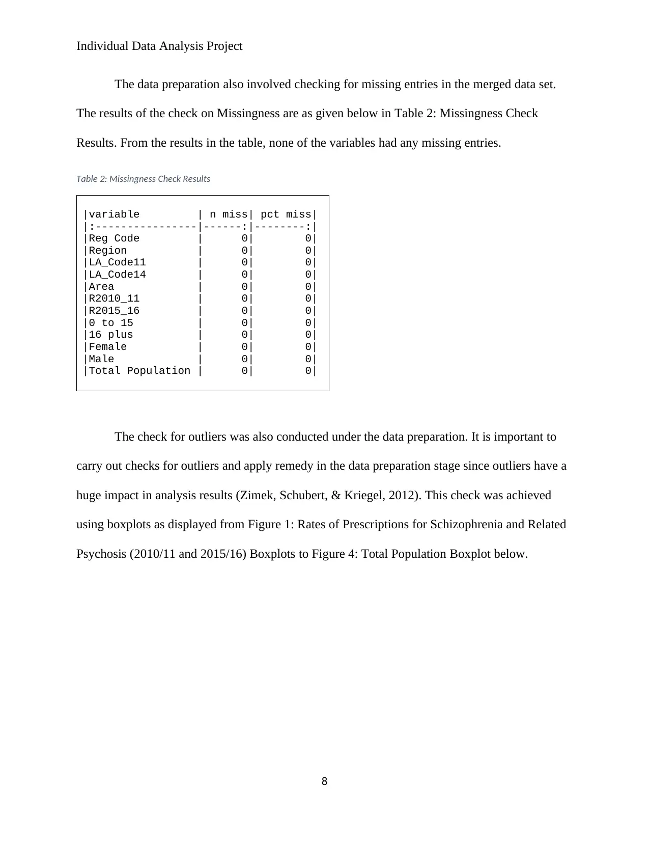
The data preparation also involved checking for missing entries in the merged data set.
The results of the check on Missingness are as given below in Table 2: Missingness Check
Results. From the results in the table, none of the variables had any missing entries.
Table 2: Missingness Check Results
|variable | n miss| pct miss|
|:----------------|------:|--------:|
|Reg Code | 0| 0|
|Region | 0| 0|
|LA_Code11 | 0| 0|
|LA_Code14 | 0| 0|
|Area | 0| 0|
|R2010_11 | 0| 0|
|R2015_16 | 0| 0|
|0 to 15 | 0| 0|
|16 plus | 0| 0|
|Female | 0| 0|
|Male | 0| 0|
|Total Population | 0| 0|
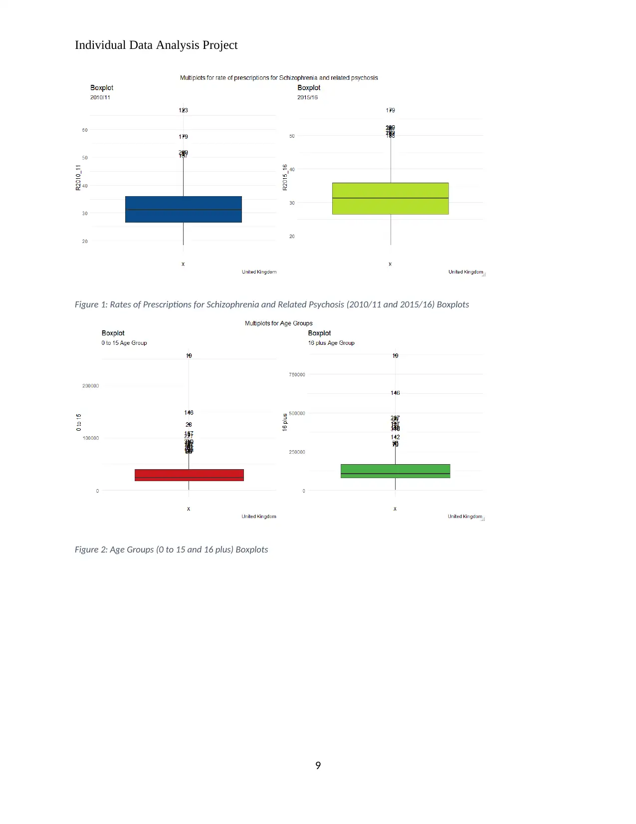
The check for outliers was also conducted under the data preparation. It is important to
carry out checks for outliers and apply remedy in the data preparation stage since outliers have a
huge impact in analysis results (Zimek, Schubert, & Kriegel, 2012). This check was achieved
using boxplots as displayed from Figure 1: Rates of Prescriptions for Schizophrenia and Related
Psychosis (2010/11 and 2015/16) Boxplots to Figure 4: Total Population Boxplot below.
8
The data preparation also involved checking for missing entries in the merged data set.
The results of the check on Missingness are as given below in Table 2: Missingness Check
Results. From the results in the table, none of the variables had any missing entries.
Table 2: Missingness Check Results
|variable | n miss| pct miss|
|:----------------|------:|--------:|
|Reg Code | 0| 0|
|Region | 0| 0|
|LA_Code11 | 0| 0|
|LA_Code14 | 0| 0|
|Area | 0| 0|
|R2010_11 | 0| 0|
|R2015_16 | 0| 0|
|0 to 15 | 0| 0|
|16 plus | 0| 0|
|Female | 0| 0|
|Male | 0| 0|
|Total Population | 0| 0|
The check for outliers was also conducted under the data preparation. It is important to
carry out checks for outliers and apply remedy in the data preparation stage since outliers have a
huge impact in analysis results (Zimek, Schubert, & Kriegel, 2012). This check was achieved
using boxplots as displayed from Figure 1: Rates of Prescriptions for Schizophrenia and Related
Psychosis (2010/11 and 2015/16) Boxplots to Figure 4: Total Population Boxplot below.
8
Individual Data Analysis Project
Figure 1: Rates of Prescriptions for Schizophrenia and Related Psychosis (2010/11 and 2015/16) Boxplots
Figure 2: Age Groups (0 to 15 and 16 plus) Boxplots
9
Figure 1: Rates of Prescriptions for Schizophrenia and Related Psychosis (2010/11 and 2015/16) Boxplots
Figure 2: Age Groups (0 to 15 and 16 plus) Boxplots
9
⊘ This is a preview!⊘
Do you want full access?
Subscribe today to unlock all pages.
Trusted by 1+ million students worldwide
Individual Data Analysis Project
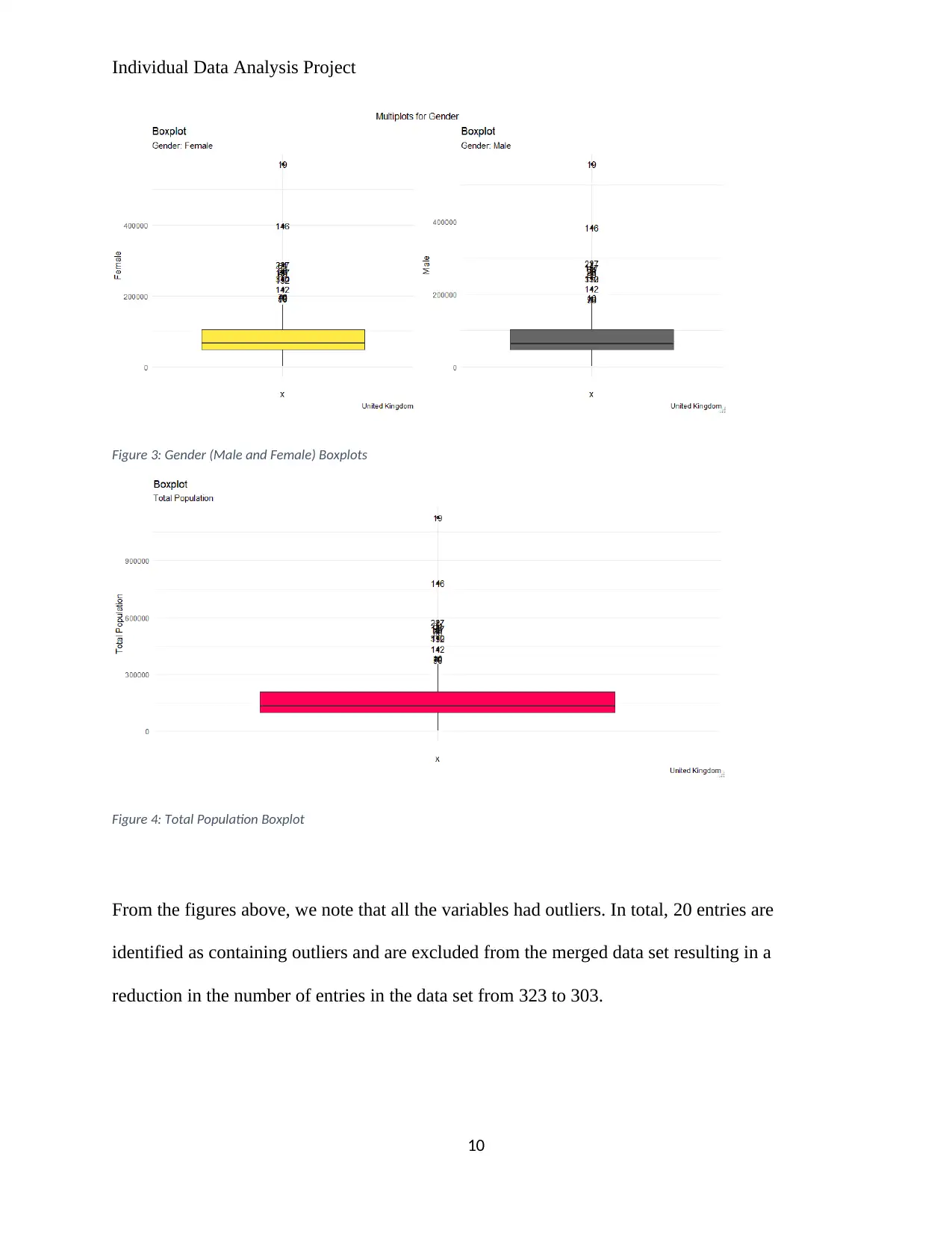
Figure 3: Gender (Male and Female) Boxplots
Figure 4: Total Population Boxplot
From the figures above, we note that all the variables had outliers. In total, 20 entries are
identified as containing outliers and are excluded from the merged data set resulting in a
reduction in the number of entries in the data set from 323 to 303.
10
Paraphrase This Document
Need a fresh take? Get an instant paraphrase of this document with our AI Paraphraser
Individual Data Analysis Project
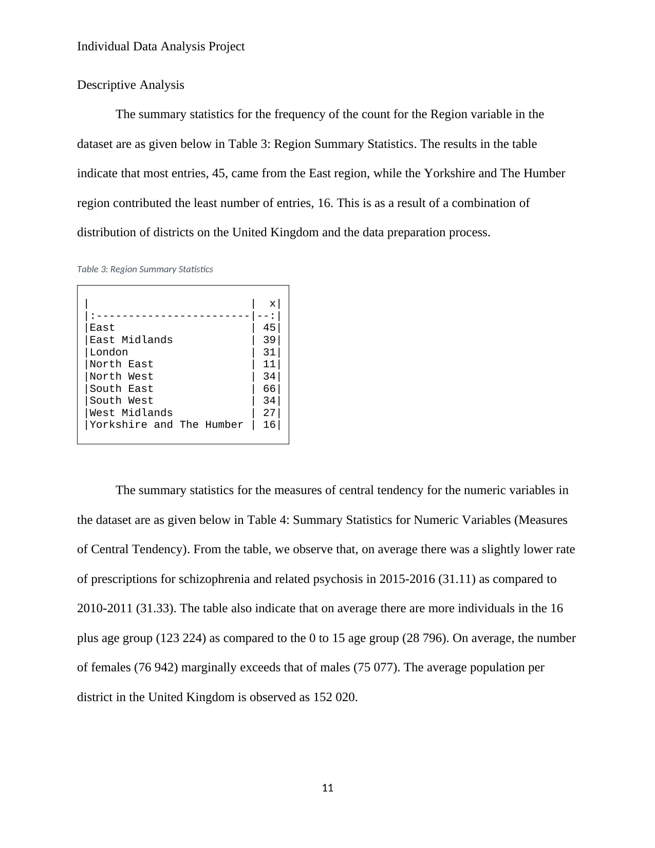
Descriptive Analysis
The summary statistics for the frequency of the count for the Region variable in the
dataset are as given below in Table 3: Region Summary Statistics. The results in the table
indicate that most entries, 45, came from the East region, while the Yorkshire and The Humber
region contributed the least number of entries, 16. This is as a result of a combination of
distribution of districts on the United Kingdom and the data preparation process.
Table 3: Region Summary Statistics
| | x|
|:------------------------|--:|
|East | 45|
|East Midlands | 39|
|London | 31|
|North East | 11|
|North West | 34|
|South East | 66|
|South West | 34|
|West Midlands | 27|
|Yorkshire and The Humber | 16|
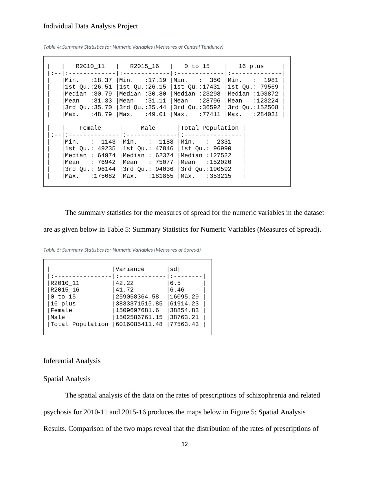
The summary statistics for the measures of central tendency for the numeric variables in
the dataset are as given below in Table 4: Summary Statistics for Numeric Variables (Measures
of Central Tendency). From the table, we observe that, on average there was a slightly lower rate
of prescriptions for schizophrenia and related psychosis in 2015-2016 (31.11) as compared to
2010-2011 (31.33). The table also indicate that on average there are more individuals in the 16
plus age group (123 224) as compared to the 0 to 15 age group (28 796). On average, the number
of females (76 942) marginally exceeds that of males (75 077). The average population per
district in the United Kingdom is observed as 152 020.
11
Descriptive Analysis
The summary statistics for the frequency of the count for the Region variable in the
dataset are as given below in Table 3: Region Summary Statistics. The results in the table
indicate that most entries, 45, came from the East region, while the Yorkshire and The Humber
region contributed the least number of entries, 16. This is as a result of a combination of
distribution of districts on the United Kingdom and the data preparation process.
Table 3: Region Summary Statistics
| | x|
|:------------------------|--:|
|East | 45|
|East Midlands | 39|
|London | 31|
|North East | 11|
|North West | 34|
|South East | 66|
|South West | 34|
|West Midlands | 27|
|Yorkshire and The Humber | 16|
The summary statistics for the measures of central tendency for the numeric variables in
the dataset are as given below in Table 4: Summary Statistics for Numeric Variables (Measures
of Central Tendency). From the table, we observe that, on average there was a slightly lower rate
of prescriptions for schizophrenia and related psychosis in 2015-2016 (31.11) as compared to
2010-2011 (31.33). The table also indicate that on average there are more individuals in the 16
plus age group (123 224) as compared to the 0 to 15 age group (28 796). On average, the number
of females (76 942) marginally exceeds that of males (75 077). The average population per
district in the United Kingdom is observed as 152 020.
11
Individual Data Analysis Project
Table 4: Summary Statistics for Numeric Variables (Measures of Central Tendency)
| | R2010_11 | R2015_16 | 0 to 15 | 16 plus |
|:--|:-------------|:-------------|:-------------|:--------------|
| |Min. :18.37 |Min. :17.19 |Min. : 350 |Min. : 1981 |
| |1st Qu.:26.51 |1st Qu.:26.15 |1st Qu.:17431 |1st Qu.: 79569 |
| |Median :30.79 |Median :30.80 |Median :23298 |Median :103872 |
| |Mean :31.33 |Mean :31.11 |Mean :28796 |Mean :123224 |
| |3rd Qu.:35.70 |3rd Qu.:35.44 |3rd Qu.:36592 |3rd Qu.:152508 |
| |Max. :48.79 |Max. :49.01 |Max. :77411 |Max. :284031 |
| | Female | Male |Total Population |
|:--|:--------------|:--------------|:----------------|
| |Min. : 1143 |Min. : 1188 |Min. : 2331 |
| |1st Qu.: 49235 |1st Qu.: 47846 |1st Qu.: 96990 |
| |Median : 64974 |Median : 62374 |Median :127522 |
| |Mean : 76942 |Mean : 75077 |Mean :152020 |
| |3rd Qu.: 96144 |3rd Qu.: 94036 |3rd Qu.:190592 |
| |Max. :175082 |Max. :181865 |Max. :353215 |
The summary statistics for the measures of spread for the numeric variables in the dataset
are as given below in Table 5: Summary Statistics for Numeric Variables (Measures of Spread).
Table 5: Summary Statistics for Numeric Variables (Measures of Spread)
| |Variance |sd|
|:----------------|:-------------|:--------|
|R2010_11 |42.22 |6.5 |
|R2015_16 |41.72 |6.46 |
|0 to 15 |259058364.58 |16095.29 |
|16 plus |3833371515.85 |61914.23 |
|Female |1509697681.6 |38854.83 |
|Male |1502586761.15 |38763.21 |
|Total Population |6016085411.48 |77563.43 |
Inferential Analysis
Spatial Analysis
The spatial analysis of the data on the rates of prescriptions of schizophrenia and related
psychosis for 2010-11 and 2015-16 produces the maps below in Figure 5: Spatial Analysis
Results. Comparison of the two maps reveal that the distribution of the rates of prescriptions of
12
⊘ This is a preview!⊘
Do you want full access?
Subscribe today to unlock all pages.
Trusted by 1+ million students worldwide
1 out of 32
Related Documents


Your All-in-One AI-Powered Toolkit for Academic Success.
+13062052269
info@desklib.com
Available 24*7 on WhatsApp / Email
![[object Object]](/_next/static/media/star-bottom.7253800d.svg)
Unlock your academic potential
Copyright © 2020–2026 A2Z Services. All Rights Reserved. Developed and managed by ZUCOL.