Introduction to Biostatistics

This document provides an introduction to biostatistics, covering topics such as data distribution, hypothesis testing, and statistical analysis. It also includes examples and explanations of various statistical tests and their applications in healthcare and medicine.

Introduction to Biostatistics
Assignment 2
Student Name:
Student Number:
1

Question 1
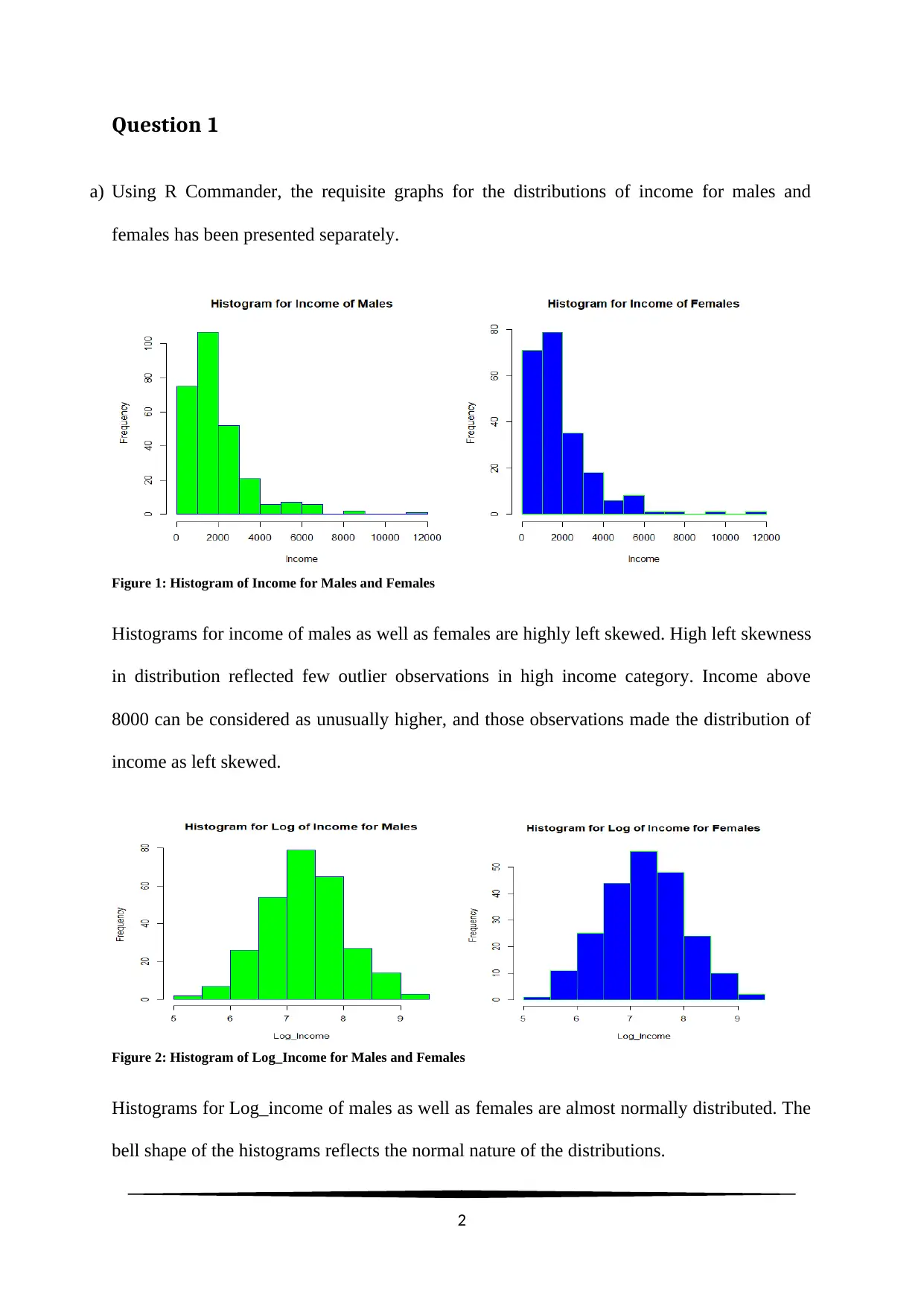
a) Using R Commander, the requisite graphs for the distributions of income for males and
females has been presented separately.
Figure 1: Histogram of Income for Males and Females
Histograms for income of males as well as females are highly left skewed. High left skewness
in distribution reflected few outlier observations in high income category. Income above
8000 can be considered as unusually higher, and those observations made the distribution of
income as left skewed.
Figure 2: Histogram of Log_Income for Males and Females
Histograms for Log_income of males as well as females are almost normally distributed. The
bell shape of the histograms reflects the normal nature of the distributions.
2

b) An independent sample t-test requires some assumptions to be satisfied. One of the
assumptions of independent t-test is normality of distribution of the sample. In this case
Log_income for both male and females are almost normally distributed. Hence, Log_income
are more appropriate compared to income for t-test.
c) Using R Commander, the results have been presented.
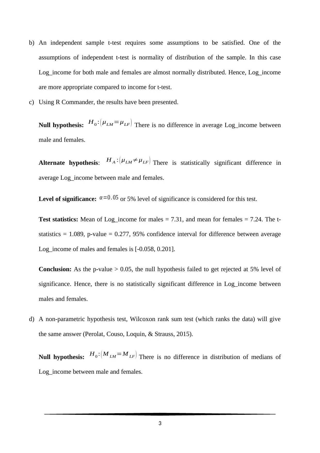
Null hypothesis: H0 : ( μLM =μLF ) There is no difference in average Log_income between
male and females.
Alternate hypothesis: H A : ( μLM ≠μLF ) There is statistically significant difference in
average Log_income between male and females.
Level of significance: α=0 . 05 or 5% level of significance is considered for this test.
Test statistics: Mean of Log_income for males = 7.31, and mean for females = 7.24. The t-
statistics = 1.089, p-value = 0.277, 95% confidence interval for difference between average
Log_income of males and females is [-0.058, 0.201].
Conclusion: As the p-value > 0.05, the null hypothesis failed to get rejected at 5% level of
significance. Hence, there is no statistically significant difference in Log_income between
males and females.
d) A non-parametric hypothesis test, Wilcoxon rank sum test (which ranks the data) will give
the same answer (Perolat, Couso, Loquin, & Strauss, 2015).
Null hypothesis: H0 : ( M LM =M LF ) There is no difference in distribution of medians of
Log_income between male and females.
3

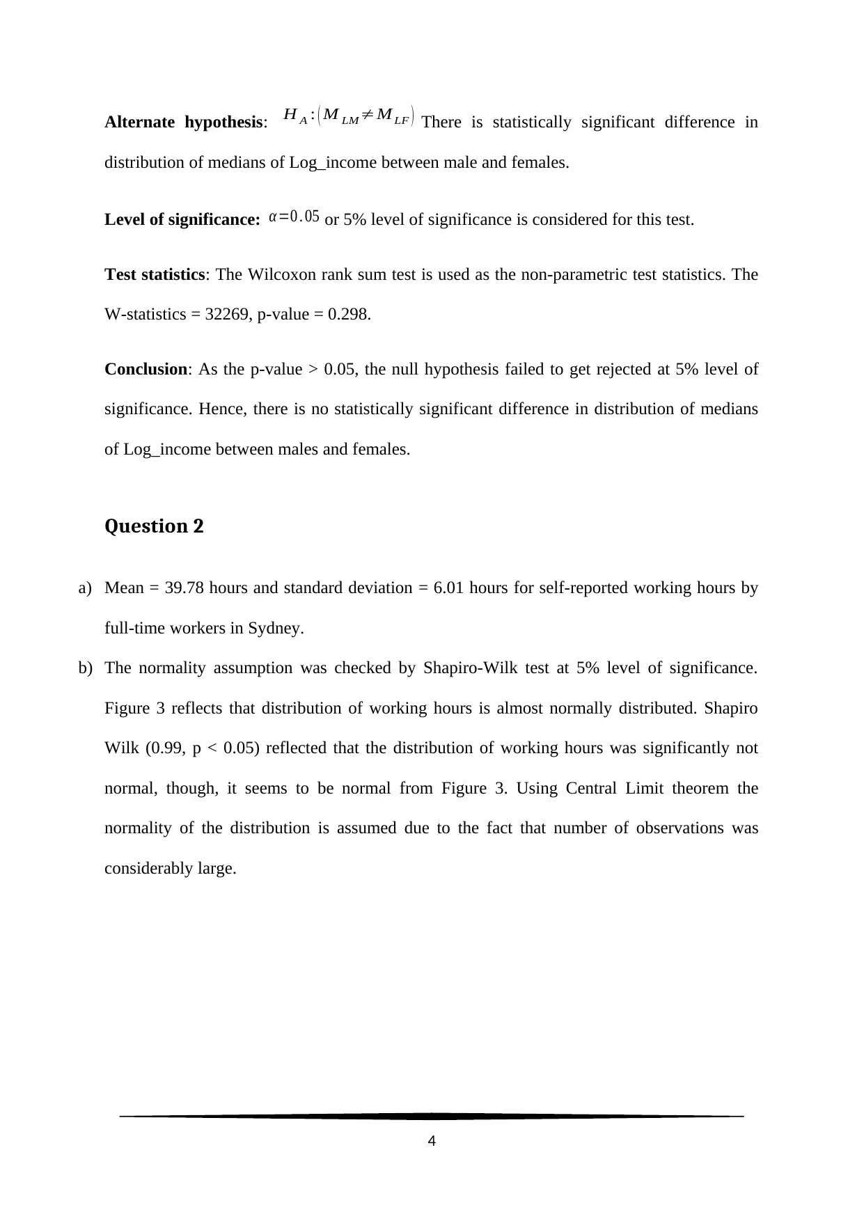
Alternate hypothesis: H A : ( M LM ≠M LF ) There is statistically significant difference in
distribution of medians of Log_income between male and females.
Level of significance: α=0 . 05 or 5% level of significance is considered for this test.
Test statistics: The Wilcoxon rank sum test is used as the non-parametric test statistics. The
W-statistics = 32269, p-value = 0.298.
Conclusion: As the p-value > 0.05, the null hypothesis failed to get rejected at 5% level of
significance. Hence, there is no statistically significant difference in distribution of medians
of Log_income between males and females.
Question 2
a) Mean = 39.78 hours and standard deviation = 6.01 hours for self-reported working hours by
full-time workers in Sydney.
b) The normality assumption was checked by Shapiro-Wilk test at 5% level of significance.
Figure 3 reflects that distribution of working hours is almost normally distributed. Shapiro
Wilk (0.99, p < 0.05) reflected that the distribution of working hours was significantly not
normal, though, it seems to be normal from Figure 3. Using Central Limit theorem the
normality of the distribution is assumed due to the fact that number of observations was
considerably large.
4

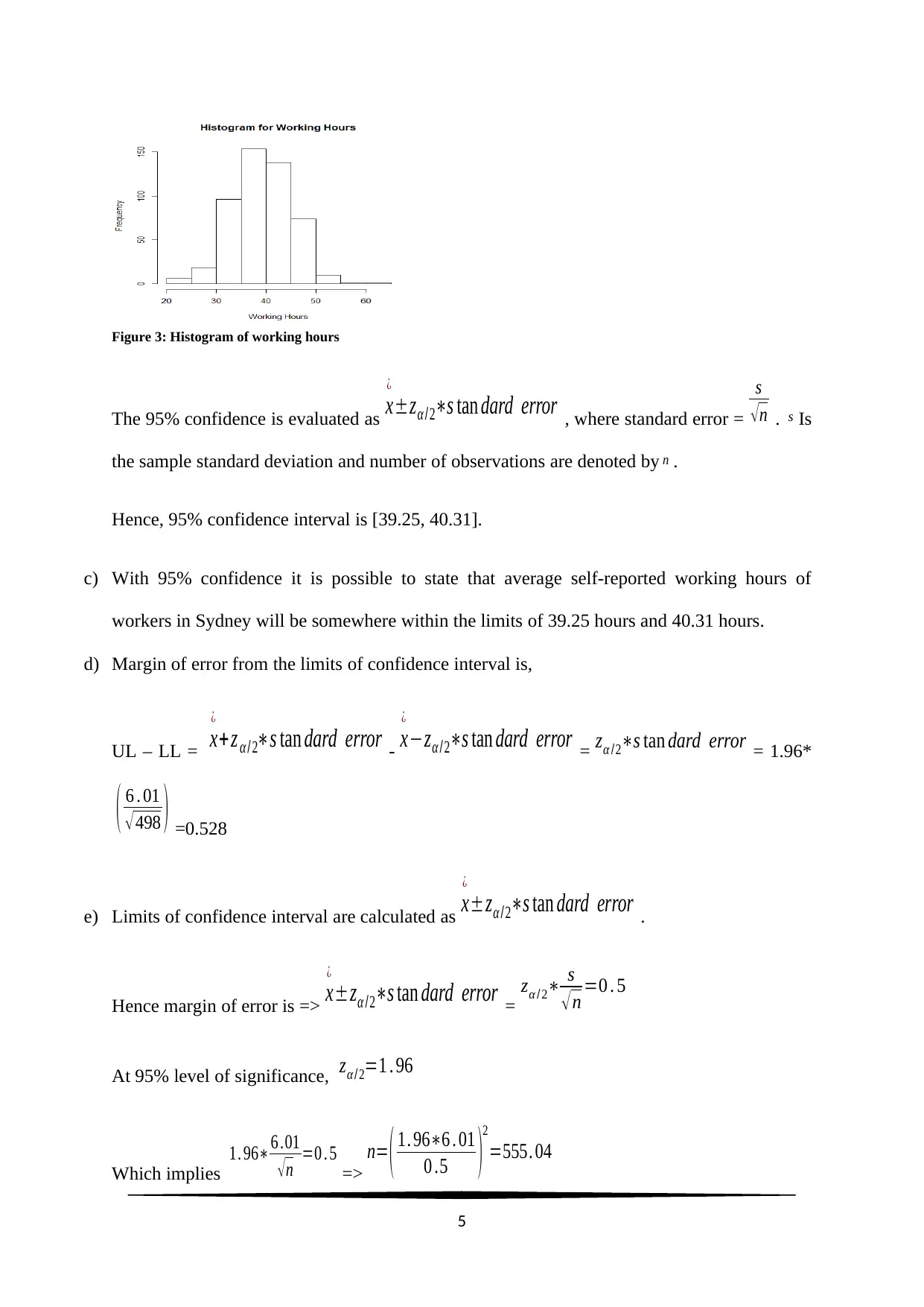
Figure 3: Histogram of working hours
The 95% confidence is evaluated as x
¿
±zα / 2∗s tan dard error , where standard error =
s
√ n . s Is
the sample standard deviation and number of observations are denoted by n .
Hence, 95% confidence interval is [39.25, 40.31].
c) With 95% confidence it is possible to state that average self-reported working hours of
workers in Sydney will be somewhere within the limits of 39.25 hours and 40.31 hours.
d) Margin of error from the limits of confidence interval is,
UL – LL = x
¿
+ z α / 2∗s tan dard error - x
¿
−zα / 2∗s tan dard error = zα /2∗s tan dard error = 1.96*
( 6 . 01
√ 498 ) =0.528
e) Limits of confidence interval are calculated as x
¿
±zα /2∗s tan dard error .
Hence margin of error is => x
¿
±zα /2∗s tan dard error =
zα /2∗ s
√ n =0 . 5
At 95% level of significance, zα /2=1 . 96
Which implies
1. 96∗6 .01
√ n =0 . 5
=>
n= ( 1. 96∗6 . 01
0 .5 )
2
=555. 04
5

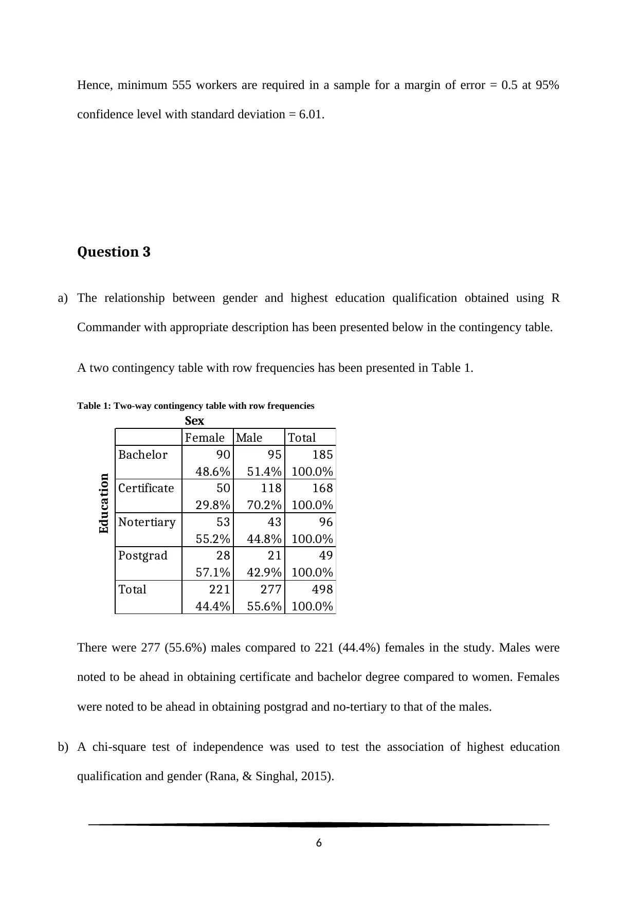
Hence, minimum 555 workers are required in a sample for a margin of error = 0.5 at 95%
confidence level with standard deviation = 6.01.
Question 3
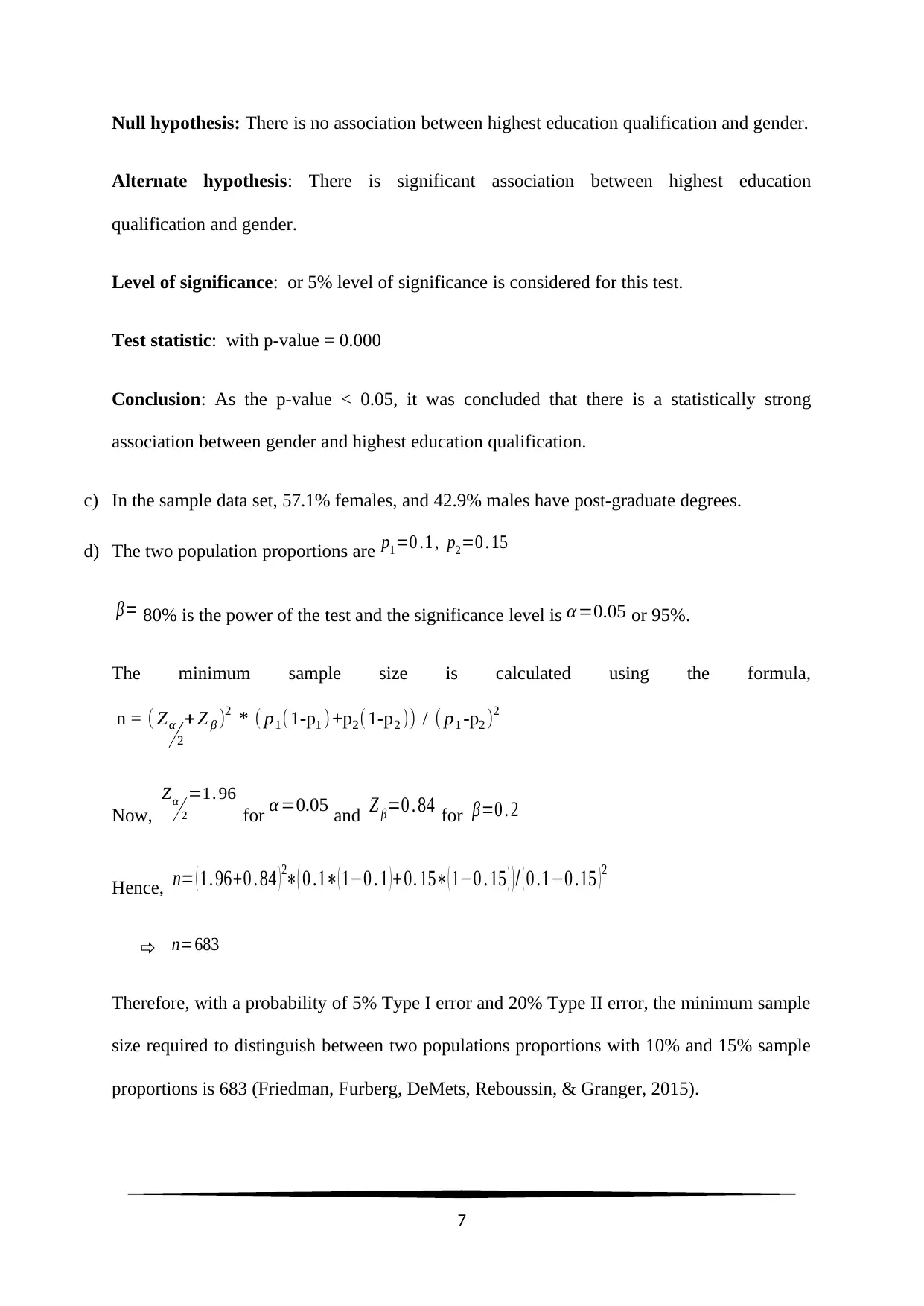
a) The relationship between gender and highest education qualification obtained using R
Commander with appropriate description has been presented below in the contingency table.
A two contingency table with row frequencies has been presented in Table 1.
Table 1: Two-way contingency table with row frequencies
Female Male Total
Bachelor 90 95 185
48.6% 51.4% 100.0%
Certificate 50 118 168
29.8% 70.2% 100.0%
Notertiary 53 43 96
55.2% 44.8% 100.0%
Postgrad 28 21 49
57.1% 42.9% 100.0%
Total 221 277 498
44.4% 55.6% 100.0%
Sex
Education
There were 277 (55.6%) males compared to 221 (44.4%) females in the study. Males were
noted to be ahead in obtaining certificate and bachelor degree compared to women. Females
were noted to be ahead in obtaining postgrad and no-tertiary to that of the males.
b) A chi-square test of independence was used to test the association of highest education
qualification and gender (Rana, & Singhal, 2015).
6

Null hypothesis: There is no association between highest education qualification and gender.
Alternate hypothesis: There is significant association between highest education
qualification and gender.
Level of significance: or 5% level of significance is considered for this test.
Test statistic: with p-value = 0.000
Conclusion: As the p-value < 0.05, it was concluded that there is a statistically strong
association between gender and highest education qualification.
c) In the sample data set, 57.1% females, and 42.9% males have post-graduate degrees.
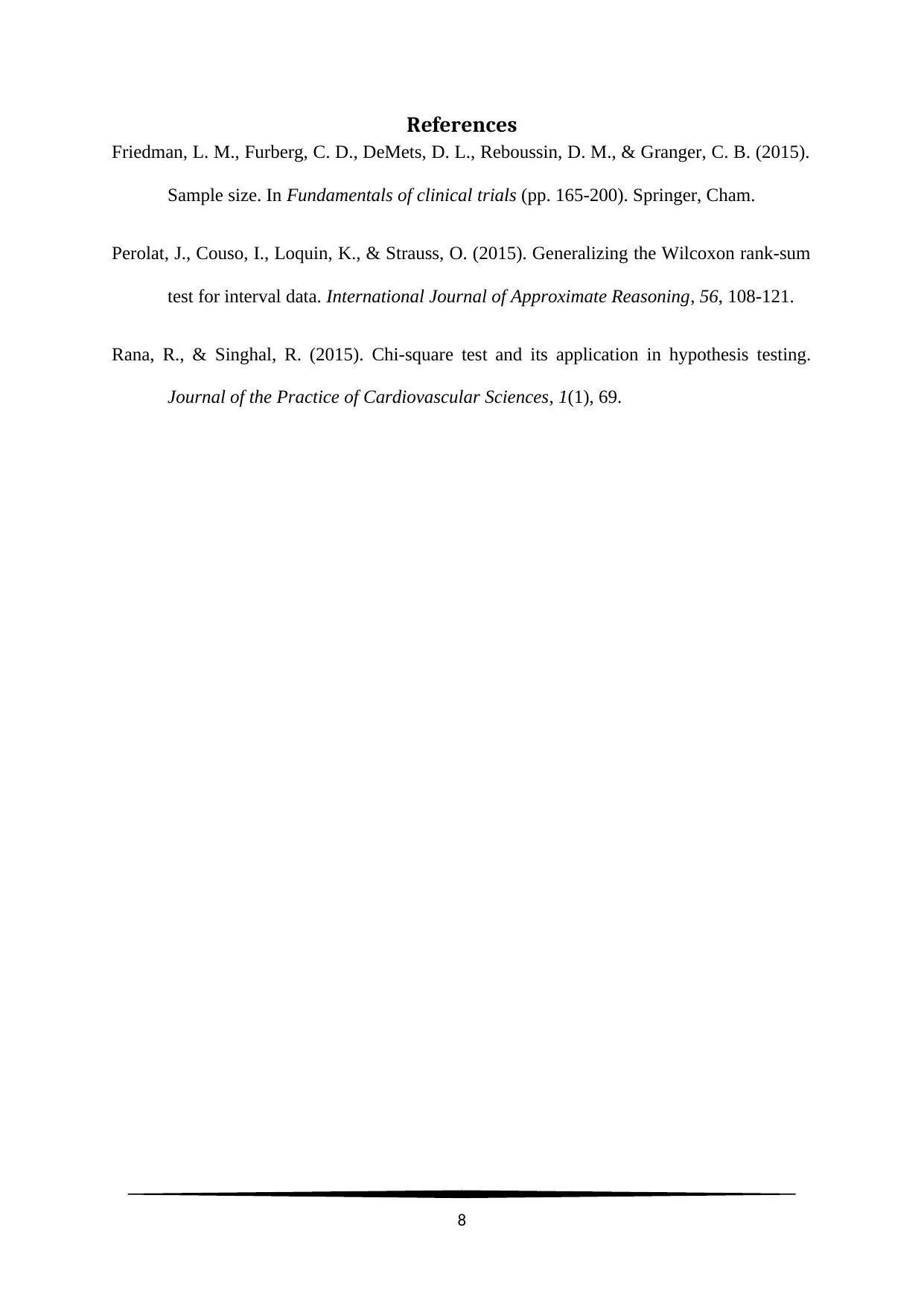
d) The two population proportions are p1=0 .1 , p2=0 . 15
β= 80% is the power of the test and the significance level is α=0.05 or 95%.
The minimum sample size is calculated using the formula,
n = ( Zα
2
+Z β )2 * ( p1(1-p1 )+p2(1-p2 )) / ( p1 -p2 )2
Now,
Zα
2
=1. 96
for α=0.05 and Z β=0 . 84 for β=0 . 2
Hence, n= ( 1. 96+0 . 84 ) 2∗( 0 .1∗( 1−0 . 1 ) + 0. 15∗( 1−0 . 15 ) ) / ( 0 .1−0 .15 ) 2
 n=683
Therefore, with a probability of 5% Type I error and 20% Type II error, the minimum sample
size required to distinguish between two populations proportions with 10% and 15% sample
proportions is 683 (Friedman, Furberg, DeMets, Reboussin, & Granger, 2015).
7

References
Friedman, L. M., Furberg, C. D., DeMets, D. L., Reboussin, D. M., & Granger, C. B. (2015).
Sample size. In Fundamentals of clinical trials (pp. 165-200). Springer, Cham.
Perolat, J., Couso, I., Loquin, K., & Strauss, O. (2015). Generalizing the Wilcoxon rank-sum
test for interval data. International Journal of Approximate Reasoning, 56, 108-121.
Rana, R., & Singhal, R. (2015). Chi-square test and its application in hypothesis testing.
Journal of the Practice of Cardiovascular Sciences, 1(1), 69.
8