Introductory Economics And Analysis

Introductory Economics
Name:
Institution:

Question 1
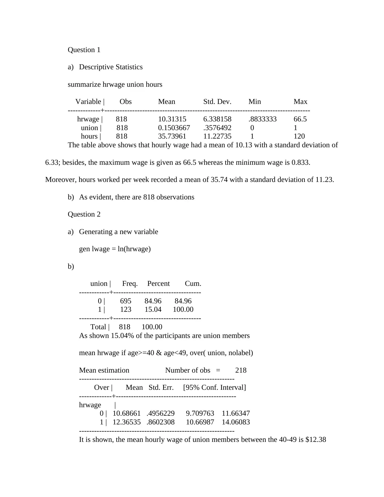
a) Descriptive Statistics
summarize hrwage union hours
Variable | Obs Mean Std. Dev. Min Max
-------------+----------------------------------------------------------------------------------
hrwage | 818 10.31315 6.338158 .8833333 66.5
union | 818 0.1503667 .3576492 0 1
hours | 818 35.73961 11.22735 1 120
The table above shows that hourly wage had a mean of 10.13 with a standard deviation of
6.33; besides, the maximum wage is given as 66.5 whereas the minimum wage is 0.833.
Moreover, hours worked per week recorded a mean of 35.74 with a standard deviation of 11.23.
b) As evident, there are 818 observations
Question 2
a) Generating a new variable
gen lwage = ln(hrwage)
b)
union | Freq. Percent Cum.
------------+-----------------------------------
0 | 695 84.96 84.96
1 | 123 15.04 100.00
------------+-----------------------------------
Total | 818 100.00
As shown 15.04% of the participants are union members
mean hrwage if age>=40 & age<49, over( union, nolabel)
Mean estimation Number of obs = 218
--------------------------------------------------------------
Over | Mean Std. Err. [95% Conf. Interval]
-------------+------------------------------------------------
hrwage |
0 | 10.68661 .4956229 9.709763 11.66347
1 | 12.36535 .8602308 10.66987 14.06083
--------------------------------------------------------------
It is shown, the mean hourly wage of union members between the 40-49 is $12.38

c) Age Group
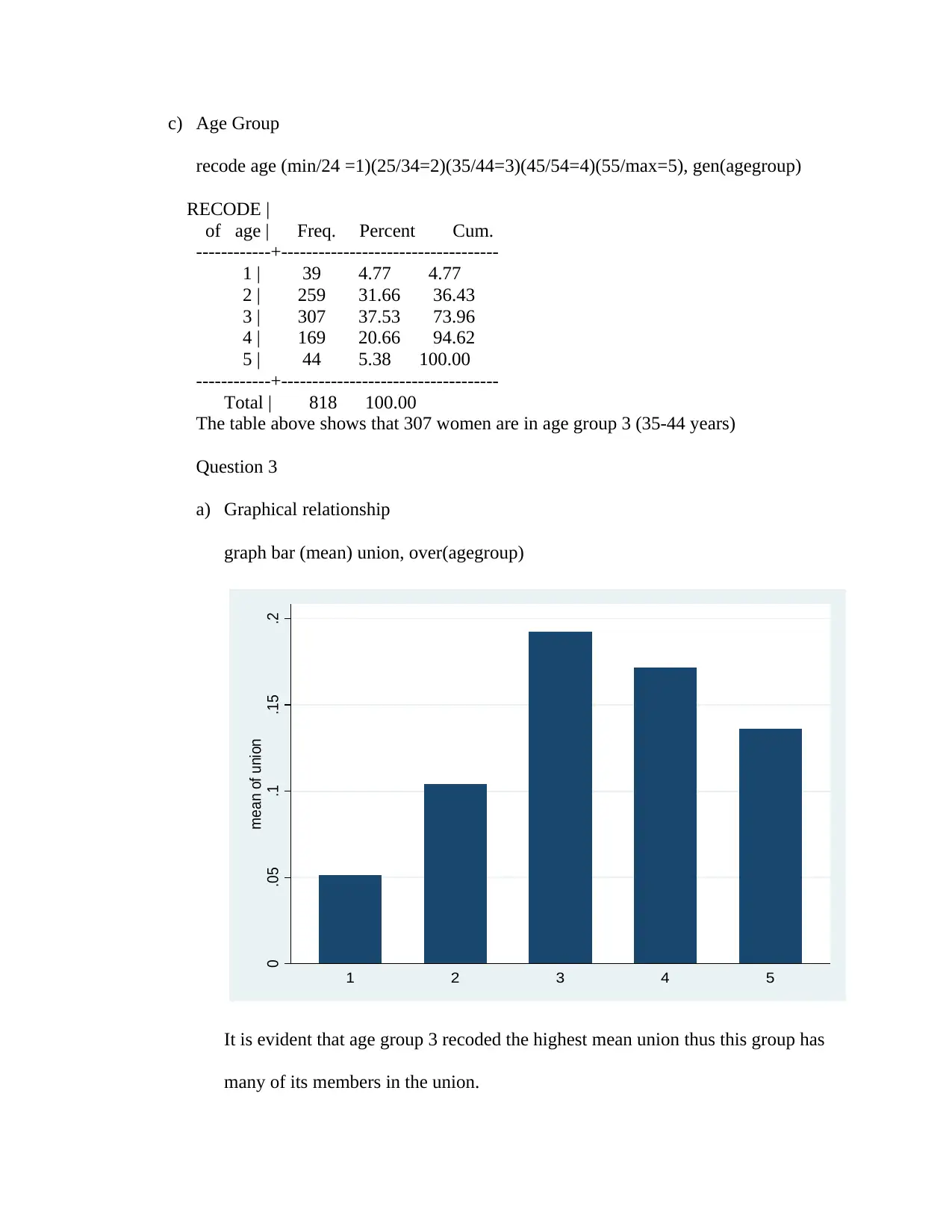
recode age (min/24 =1)(25/34=2)(35/44=3)(45/54=4)(55/max=5), gen(agegroup)
RECODE |
of age | Freq. Percent Cum.
------------+-----------------------------------
1 | 39 4.77 4.77
2 | 259 31.66 36.43
3 | 307 37.53 73.96
4 | 169 20.66 94.62
5 | 44 5.38 100.00
------------+-----------------------------------
Total | 818 100.00
The table above shows that 307 women are in age group 3 (35-44 years)
Question 3
a) Graphical relationship
graph bar (mean) union, over(agegroup)
0 .05 .1 .15 .2
mean of union
1 2 3 4 5
It is evident that age group 3 recoded the highest mean union thus this group has
many of its members in the union.

b) Correlation
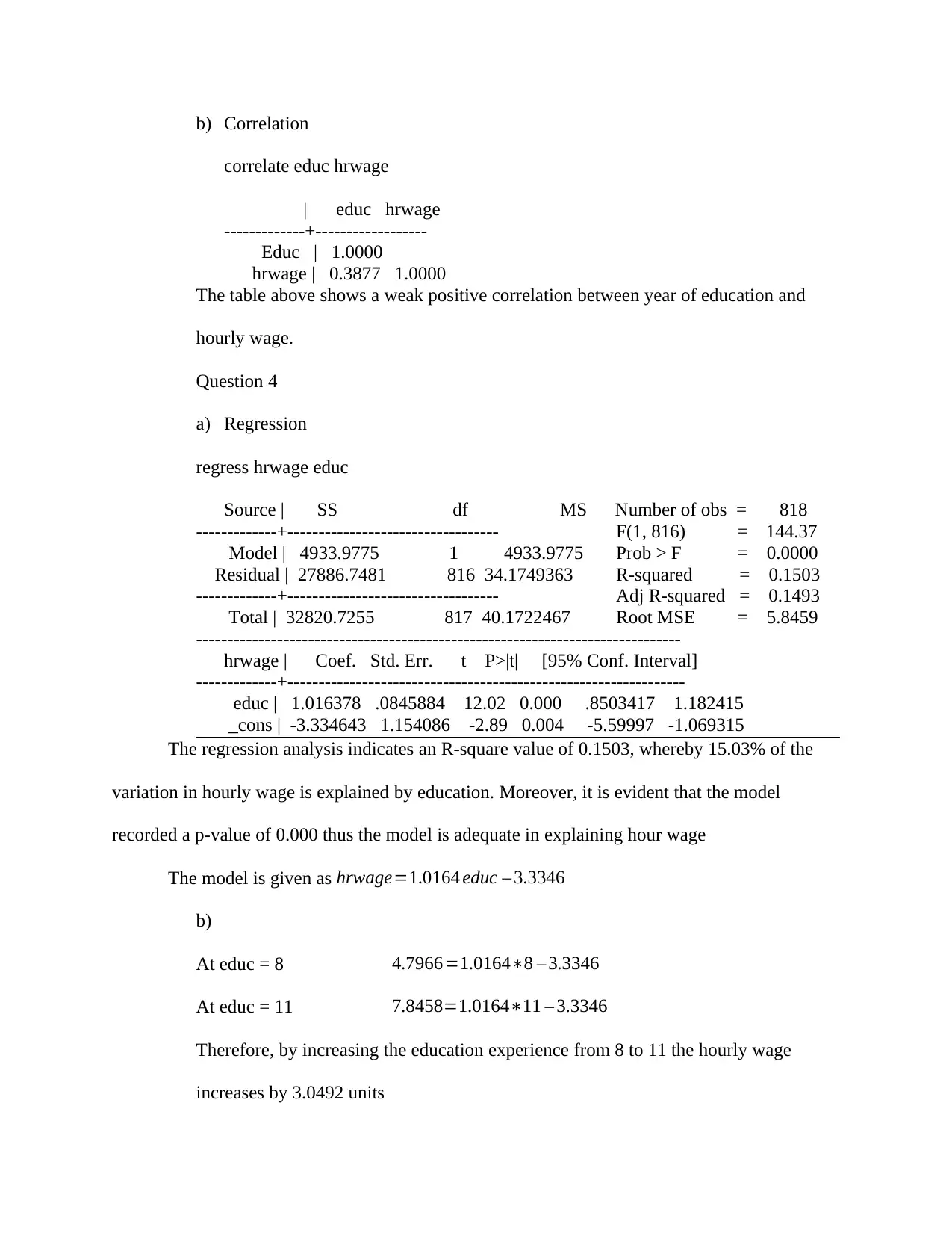
correlate educ hrwage
| educ hrwage
-------------+------------------
Educ | 1.0000
hrwage | 0.3877 1.0000
The table above shows a weak positive correlation between year of education and
hourly wage.
Question 4
a) Regression
regress hrwage educ
Source | SS df MS Number of obs = 818
-------------+---------------------------------- F(1, 816) = 144.37
Model | 4933.9775 1 4933.9775 Prob > F = 0.0000
Residual | 27886.7481 816 34.1749363 R-squared = 0.1503
-------------+---------------------------------- Adj R-squared = 0.1493
Total | 32820.7255 817 40.1722467 Root MSE = 5.8459
------------------------------------------------------------------------------
hrwage | Coef. Std. Err. t P>|t| [95% Conf. Interval]
-------------+----------------------------------------------------------------
educ | 1.016378 .0845884 12.02 0.000 .8503417 1.182415
_cons | -3.334643 1.154086 -2.89 0.004 -5.59997 -1.069315
The regression analysis indicates an R-square value of 0.1503, whereby 15.03% of the
variation in hourly wage is explained by education. Moreover, it is evident that the model
recorded a p-value of 0.000 thus the model is adequate in explaining hour wage
The model is given as hrwage=1.0164 educ – 3.3346
b)
At educ = 8 4.7966=1.0164∗8 – 3.3346
At educ = 11 7.8458=1.0164∗11 – 3.3346
Therefore, by increasing the education experience from 8 to 11 the hourly wage
increases by 3.0492 units

c)
At educ = 12 8.8622=1.0164∗8 – 3.3346
At educ = 15 11.9114=1.0164∗11 – 3.3346
Therefore, by increasing the education experience from 12 to 15 the hourly wage
increases by 3.0492 units
Question 5
a) Generating a new variable
gen exper = age - educ - 6.
b) Regression
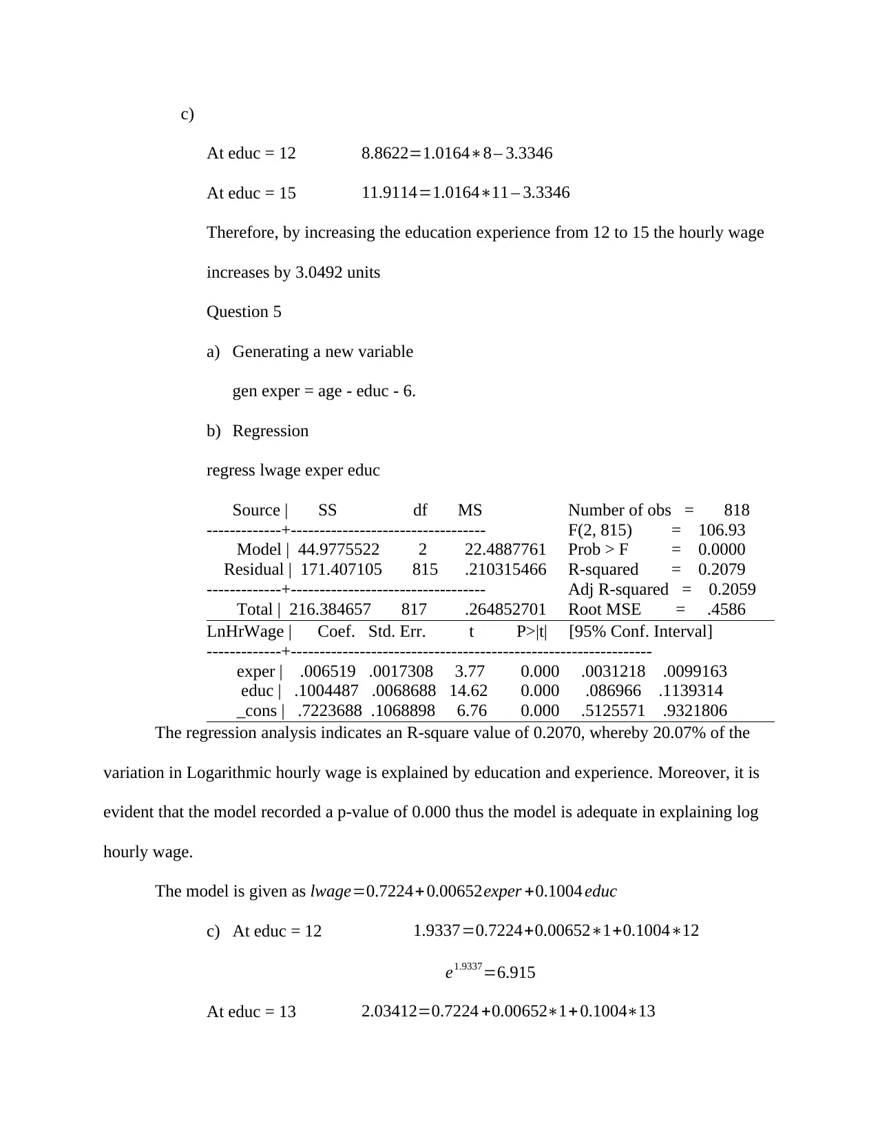
regress lwage exper educ
Source | SS df MS Number of obs = 818
-------------+---------------------------------- F(2, 815) = 106.93
Model | 44.9775522 2 22.4887761 Prob > F = 0.0000
Residual | 171.407105 815 .210315466 R-squared = 0.2079
-------------+---------------------------------- Adj R-squared = 0.2059
Total | 216.384657 817 .264852701 Root MSE = .4586
LnHrWage | Coef. Std. Err. t P>|t| [95% Conf. Interval]
-------------+---------------------------------------------------------------
exper | .006519 .0017308 3.77 0.000 .0031218 .0099163
educ | .1004487 .0068688 14.62 0.000 .086966 .1139314
_cons | .7223688 .1068898 6.76 0.000 .5125571 .9321806
The regression analysis indicates an R-square value of 0.2070, whereby 20.07% of the
variation in Logarithmic hourly wage is explained by education and experience. Moreover, it is
evident that the model recorded a p-value of 0.000 thus the model is adequate in explaining log
hourly wage.
The model is given as lwage=0.7224+ 0.00652exper +0.1004 educ
c) At educ = 12 1.9337=0.7224+0.00652∗1+0.1004∗12
e1.9337=6.915
At educ = 13 2.03412=0.7224 +0.00652∗1+0.1004∗13

e2.03412=7.6455
Therefore, by increasing the education experience from 12 to 13 the hourly wage
increases by 0.7305 units
d)
At educ = 8 1.9337=0.7224+0.00652∗1+0.1004∗9
e1.9337=4.6279
At educ = 9 2.03412=0.7224 +0.00652∗1+0.1004∗13
e2.03412=5.1167
Therefore, by increasing the education experience from 12 to 13 the hourly wage
increases by 0.4888 units
Question 6
a) Generating variable and Regression
gen expersq = exper*exper
regress lwage expersq exper educ
Source | SS df MS Number of obs = 818
-------------+---------------------------------- F(3, 814) = 71.72
Model | 45.2398026 3 15.0799342 Prob > F = 0.0000
Residual | 171.144854 814 0.210251664 R-squared = 0.2091
-------------+---------------------------------- Adj R-squared = 0.2062
Total | 216.384657 817 0.264852701 Root MSE = .45853
LnHrWage | Coef. Std. Err. t P>|t| [95% Conf. Interval]
-------------+----------------------------------------------------------------
expersq | -.0001773 .0001587 -1.12 0.264 -.0004889 .0001343
exper | .0138167 .0067595 2.04 0.041 .0005486 .0270848
educ | .0995536 .0069144 14.40 0.000 .0859814 .1131257
_cons | .6759981 .1146554 5.90 0.000 .450943 .9010532
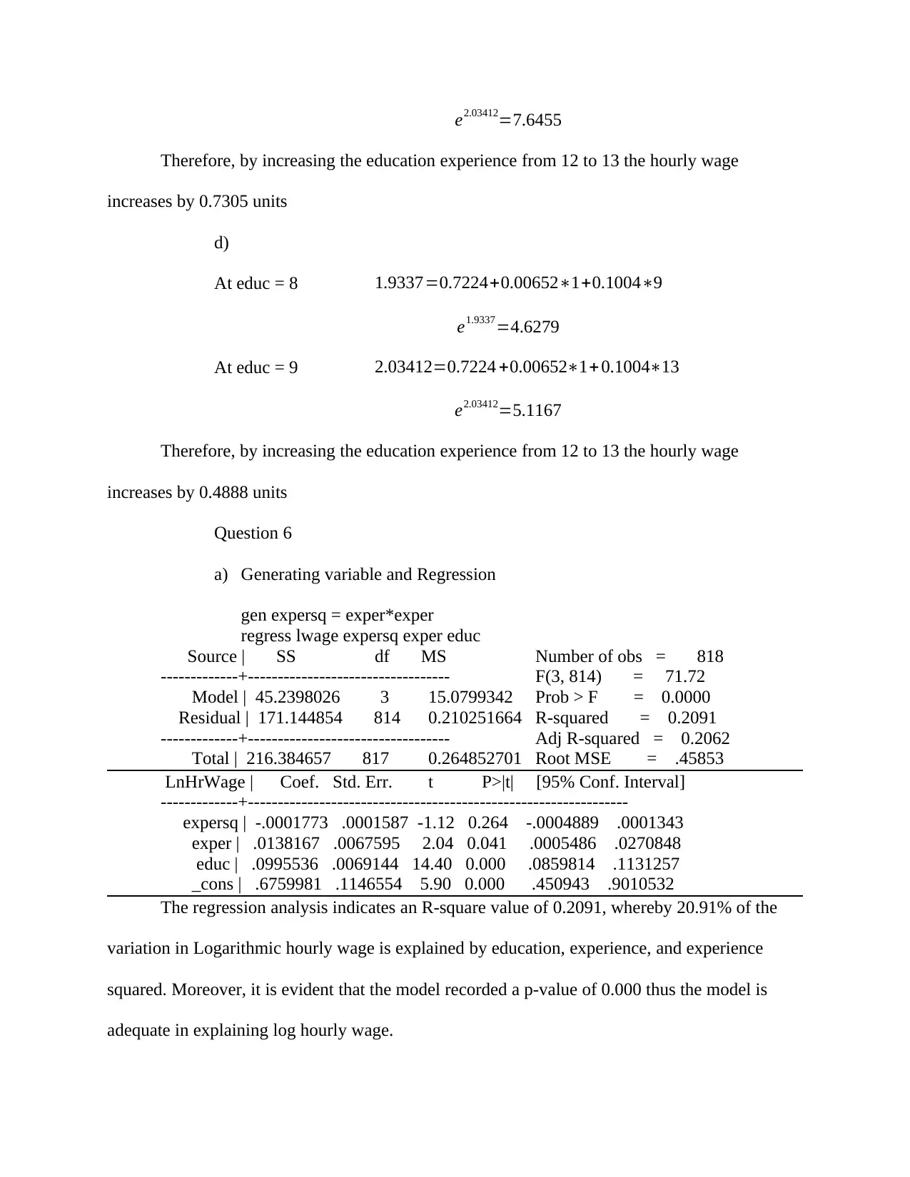
The regression analysis indicates an R-square value of 0.2091, whereby 20.91% of the
variation in Logarithmic hourly wage is explained by education, experience, and experience
squared. Moreover, it is evident that the model recorded a p-value of 0.000 thus the model is
adequate in explaining log hourly wage.

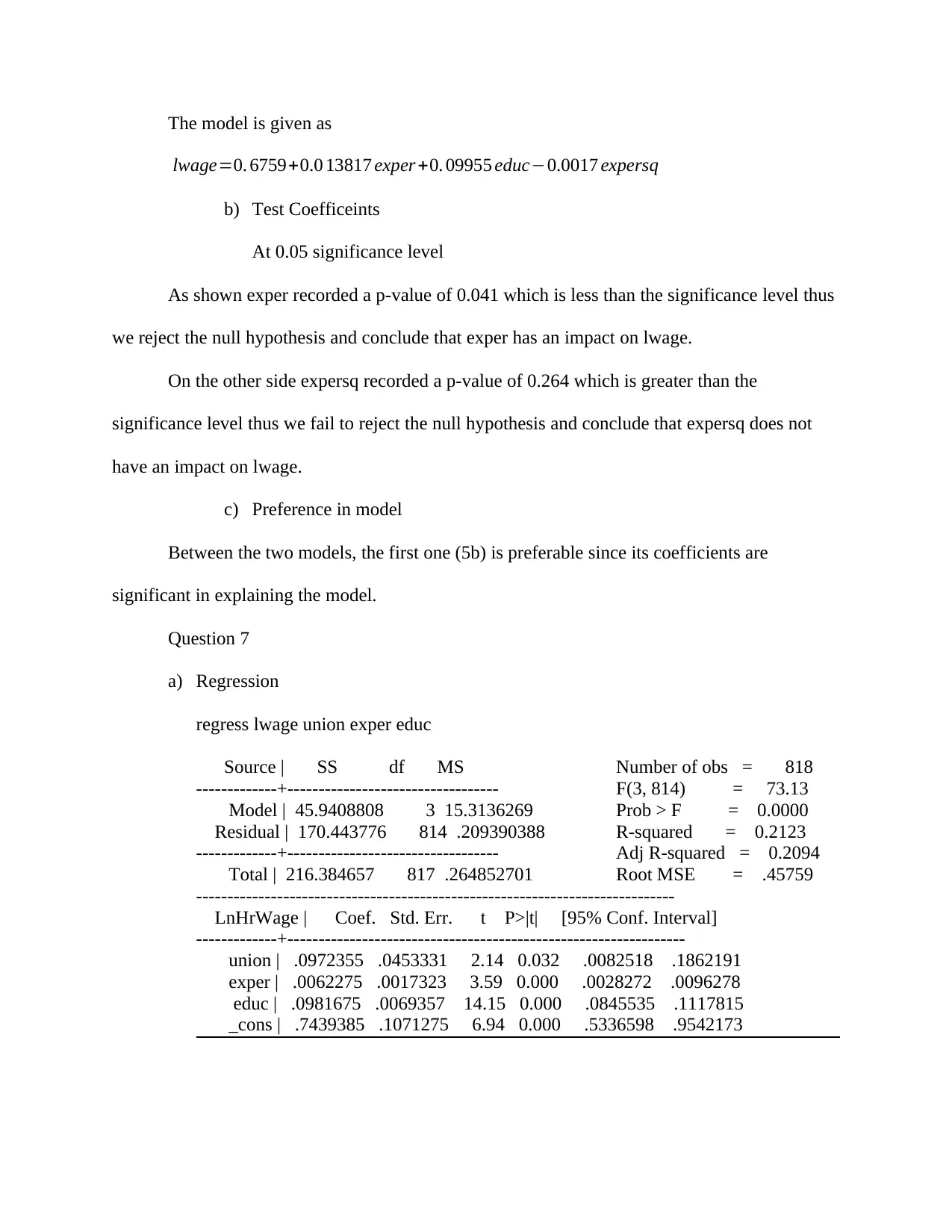
The model is given as
lwage=0. 6759+0.0 13817 exper +0. 09955 educ−0.0017 expersq
b) Test Coefficeints
At 0.05 significance level
As shown exper recorded a p-value of 0.041 which is less than the significance level thus
we reject the null hypothesis and conclude that exper has an impact on lwage.
On the other side expersq recorded a p-value of 0.264 which is greater than the
significance level thus we fail to reject the null hypothesis and conclude that expersq does not
have an impact on lwage.
c) Preference in model
Between the two models, the first one (5b) is preferable since its coefficients are
significant in explaining the model.
Question 7
a) Regression
regress lwage union exper educ
Source | SS df MS Number of obs = 818
-------------+---------------------------------- F(3, 814) = 73.13
Model | 45.9408808 3 15.3136269 Prob > F = 0.0000
Residual | 170.443776 814 .209390388 R-squared = 0.2123
-------------+---------------------------------- Adj R-squared = 0.2094
Total | 216.384657 817 .264852701 Root MSE = .45759
-----------------------------------------------------------------------------
LnHrWage | Coef. Std. Err. t P>|t| [95% Conf. Interval]
-------------+----------------------------------------------------------------
union | .0972355 .0453331 2.14 0.032 .0082518 .1862191
exper | .0062275 .0017323 3.59 0.000 .0028272 .0096278
educ | .0981675 .0069357 14.15 0.000 .0845535 .1117815
_cons | .7439385 .1071275 6.94 0.000 .5336598 .9542173

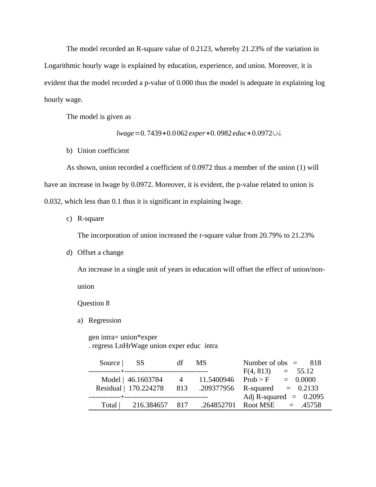
The model recorded an R-square value of 0.2123, whereby 21.23% of the variation in
Logarithmic hourly wage is explained by education, experience, and union. Moreover, it is
evident that the model recorded a p-value of 0.000 thus the model is adequate in explaining log
hourly wage.
The model is given as
lwage=0. 7439+0.0 062 exper +0. 0982 educ+0.0972∪¿
b) Union coefficient
As shown, union recorded a coefficient of 0.0972 thus a member of the union (1) will
have an increase in lwage by 0.0972. Moreover, it is evident, the p-value related to union is
0.032, which less than 0.1 thus it is significant in explaining lwage.
c) R-square
The incorporation of union increased the r-square value from 20.79% to 21.23%
d) Offset a change
An increase in a single unit of years in education will offset the effect of union/non-
union
Question 8
a) Regression
gen intra= union*exper
. regress LnHrWage union exper educ intra
Source | SS df MS Number of obs = 818
-------------+---------------------------------- F(4, 813) = 55.12
Model | 46.1603784 4 11.5400946 Prob > F = 0.0000
Residual | 170.224278 813 .209377956 R-squared = 0.2133
-------------+---------------------------------- Adj R-squared = 0.2095
Total | 216.384657 817 .264852701 Root MSE = .45758

LnHrWage | Coef. Std. Err. t P>|t| [95% Conf. Interval]
-------------+----------------------------------------------------------------
union | .2025771 .1124288 1.80 0.072 -.0181078 .4232619
exper | .0068451 .0018343 3.73 0.000 .0032447 .0104456
educ | .0980612 .0069363 14.14 0.000 .084446 .1116764
intra | -.0053035 .0051798 -1.02 0.306 -.0154708 .0048638
_cons | .7336728 .1075925 6.82 0.000 .5224809 .9448647
------------------------------------------------------------------------------
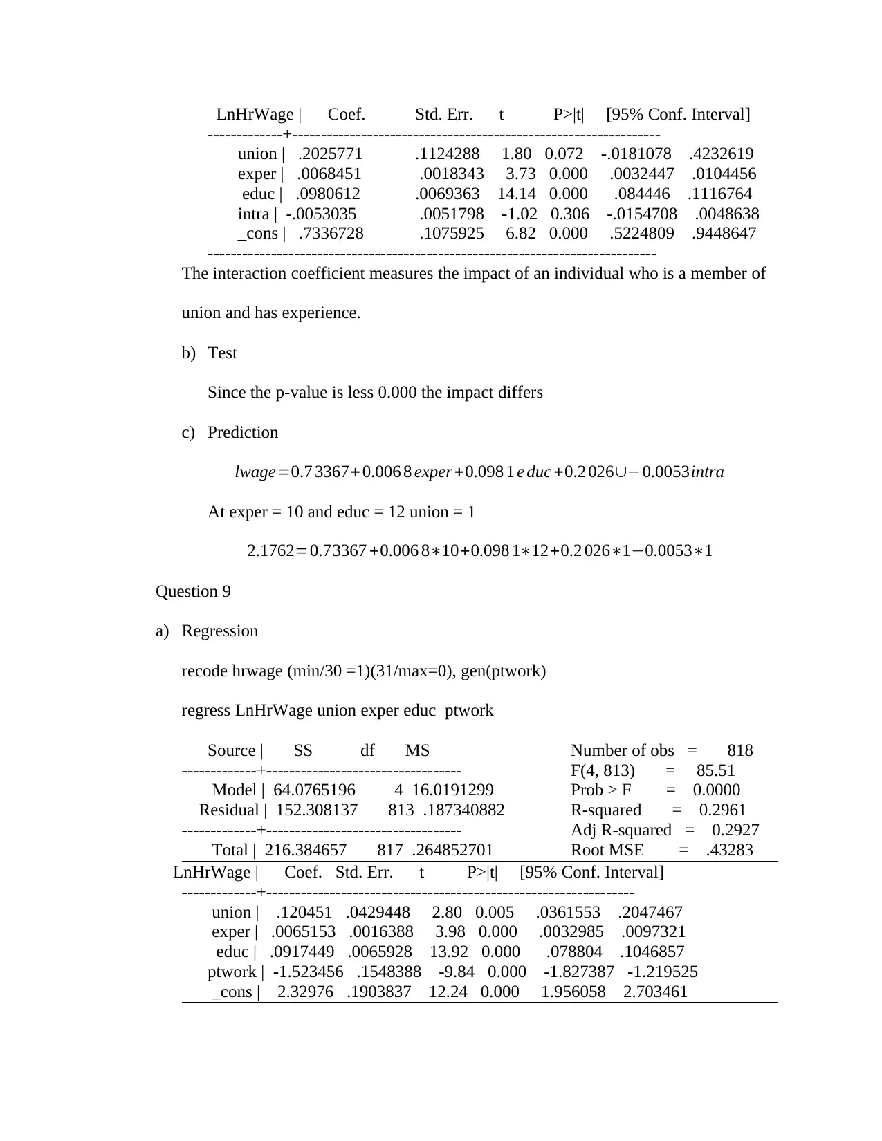
The interaction coefficient measures the impact of an individual who is a member of
union and has experience.
b) Test
Since the p-value is less 0.000 the impact differs
c) Prediction
lwage=0.7 3367+0.006 8 exper +0.098 1 e duc +0.2 026∪−0.0053intra
At exper = 10 and educ = 12 union = 1
2.1762=0.73367 +0.006 8∗10+0.098 1∗12+0.2 026∗1−0.0053∗1
Question 9
a) Regression
recode hrwage (min/30 =1)(31/max=0), gen(ptwork)
regress LnHrWage union exper educ ptwork
Source | SS df MS Number of obs = 818
-------------+---------------------------------- F(4, 813) = 85.51
Model | 64.0765196 4 16.0191299 Prob > F = 0.0000
Residual | 152.308137 813 .187340882 R-squared = 0.2961
-------------+---------------------------------- Adj R-squared = 0.2927
Total | 216.384657 817 .264852701 Root MSE = .43283
LnHrWage | Coef. Std. Err. t P>|t| [95% Conf. Interval]
-------------+----------------------------------------------------------------
union | .120451 .0429448 2.80 0.005 .0361553 .2047467
exper | .0065153 .0016388 3.98 0.000 .0032985 .0097321
educ | .0917449 .0065928 13.92 0.000 .078804 .1046857
ptwork | -1.523456 .1548388 -9.84 0.000 -1.827387 -1.219525
_cons | 2.32976 .1903837 12.24 0.000 1.956058 2.703461

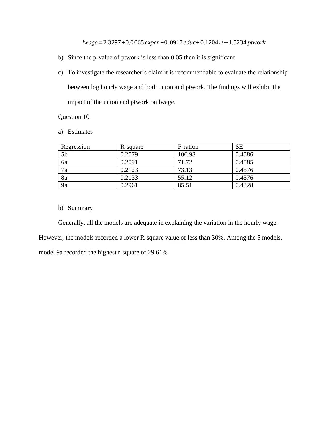
lwage=2.3297+0.0 065 exper +0. 0917 educ+ 0.1204∪−1.5234 ptwork
b) Since the p-value of ptwork is less than 0.05 then it is significant
c) To investigate the researcher’s claim it is recommendable to evaluate the relationship
between log hourly wage and both union and ptwork. The findings will exhibit the
impact of the union and ptwork on lwage.
Question 10
a) Estimates
Regression R-square F-ration SE
5b 0.2079 106.93 0.4586
6a 0.2091 71.72 0.4585
7a 0.2123 73.13 0.4576
8a 0.2133 55.12 0.4576
9a 0.2961 85.51 0.4328
b) Summary
Generally, all the models are adequate in explaining the variation in the hourly wage.
However, the models recorded a lower R-square value of less than 30%. Among the 5 models,
model 9a recorded the highest r-square of 29.61%