Quantitative Methods in Business: Inventory Control, Transportation, Distribution and Network Model

This document covers topics related to Inventory Control, Transportation, and Distribution and Network Model in Quantitative Methods in Business. It includes methods like Linear Programming, Northwest Corner Rule, and Stepping Stone Method.

Assignment 3: Quantitative Methods in
Business

Table of Contents
Question 1: Inventory Control...................................................................................................3
Question 2: Transportation.........................................................................................................5
Solution by applying Northwest Corner Rule........................................................................7
Solution by applying stepping stone method.........................................................................7
Question 3: Distribution and network model...........................................................................10
References................................................................................................................................12

QUESTION 1: INVENTORY CONTROL
Inventory control can be broadly defined as procedure relating to assessment and evaluation
of the inventory of company. The main objective of the inventory control is to maximize the
profit by maintaining the minimum inventory (Larsen, and Thorstenson, 2014). Inventory
control also known as stock control which involves the procedure of coordination and the
supervision of the supply, distribution, storage , and recording of the raw material to maintain
stock sufficient in accordance with requirement of business (Garrido-Jurado& et.al 2016).
Thus, inventory control assists the company to avoid excessive stock of its products so that
cost of maintaining the stock can be minimized. There are several methods of inventory
control which assists in determining the optimum level of inventory. Linear Programming
method is one of the best techniques which is applied for ascertaining the optimum level of
inventory (Gleixner, Steffy, and Wolter, 2016).
Linear programming method presents the comprehensive connections through the linear
functions and then assesses the optimum points. There are some common terms, which are
used in this method and same have been discussed defined below –
Decision Variable
The result of discussed issue is determined through application of the decision variable. They
reflect the ultimate outcome. In order to address any problem, it is necessary to ascertain the
decision variable on mandatory basis (Dokeroglu, 2015).
Objective function
It can be referred as goal of making decision. In the given problem, the company wants to
maximize its profit. It is denoted by Z. thus, the objective function of the current problem is
maximization of profit (Ma, and Saunders, 2015).
Constraints
The decision variable of the problem is limited or restricted by the constraints. Generally,
they restrict (limit) the value of the decision variable. In the given problem, advertising
budget, square footage and rental limits are constraints.
Non-Negativity limitation

In Linear Programming Method, the non-negativity limitation must be satisfied. In other
words, it can be said that values of the decision variable must be 0 or more than 0.
In order to solve Linear Programming problem, simplex method is one of the most
appropriate method. For solving the problem through the simplex method, objective function
is required. The objective may be maximization of the profit or the minimization of the cost
which depends on the nature of problem (METLO, SOLANGI, and MEMON, 2016). Present
discussed problem is related with the maximization of the profit. There are one or more
constraints in the problem, which represents the real value number. It is required to put the
problem in the standard manner. The inequalities in the constraints should be modified
through inserting slack or the surplus variable in the equation (Bisht, and Srivastava, 2017).
The new variables present about the unutilized capacity of the company. After this, the
problem should be arranged in the matrix form and objective function is required to added at
the bottom of the matrix. The first step of this method is to find out the initial basic feasible
solution by allocating zero values to the decision variable. It is also known as initial simplex
table. Thus, optimum solution is attained after accomplishment of test of optimality and test
of feasibility (Reyes, Solano-Charris, and Montoya-Torres, 2019).
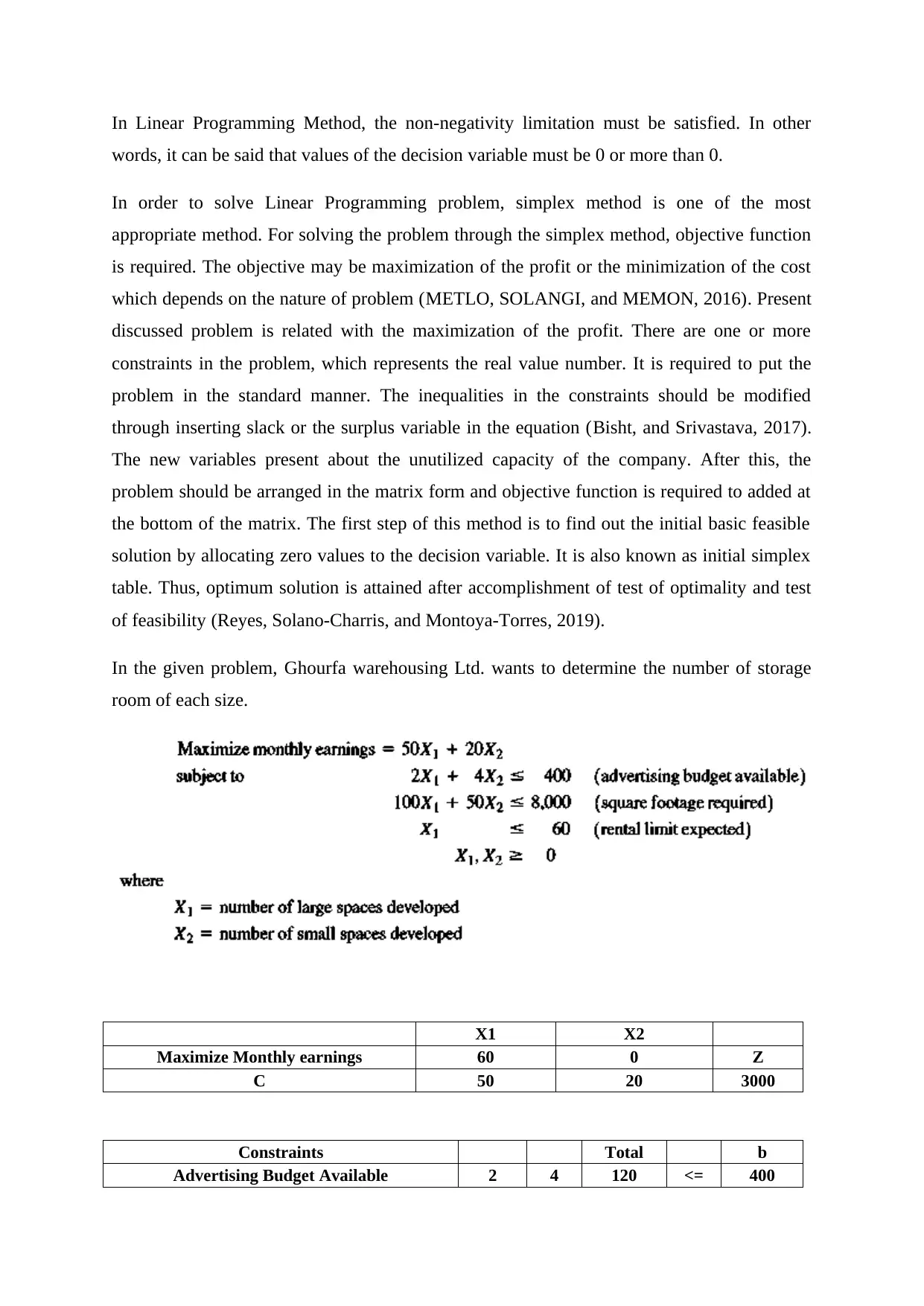
In the given problem, Ghourfa warehousing Ltd. wants to determine the number of storage
room of each size.
X1 X2
Maximize Monthly earnings 60 0 Z
C 50 20 3000
Constraints Total b
Advertising Budget Available 2 4 120 <= 400

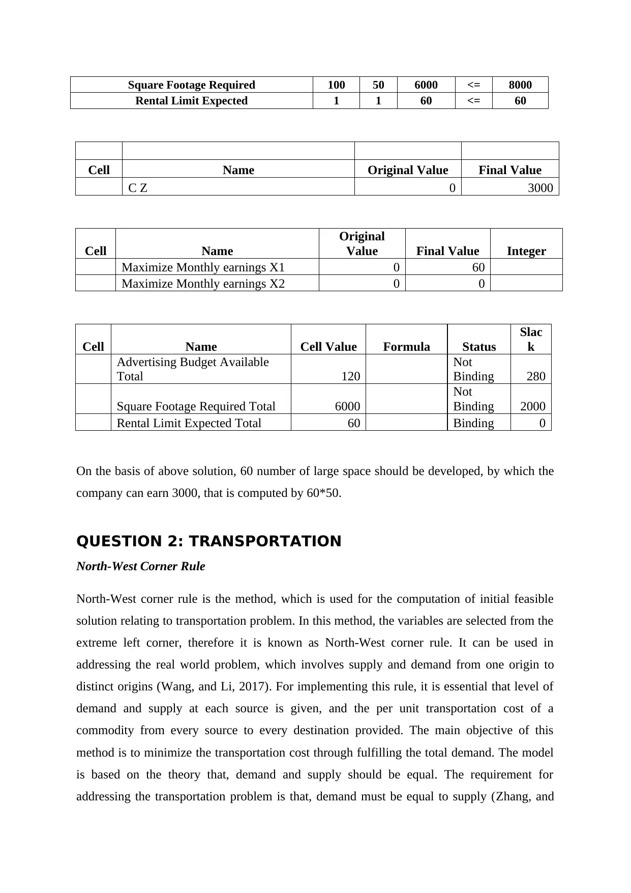
Square Footage Required 100 50 6000 <= 8000
Rental Limit Expected 1 1 60 <= 60
Cell Name Original Value Final Value
C Z 0 3000
Cell Name
Original
Value Final Value Integer
Maximize Monthly earnings X1 0 60
Maximize Monthly earnings X2 0 0
Cell Name Cell Value Formula Status
Slac
k
Advertising Budget Available
Total 120
Not
Binding 280
Square Footage Required Total 6000
Not
Binding 2000
Rental Limit Expected Total 60 Binding 0
On the basis of above solution, 60 number of large space should be developed, by which the
company can earn 3000, that is computed by 60*50.
QUESTION 2: TRANSPORTATION
North-West Corner Rule
North-West corner rule is the method, which is used for the computation of initial feasible
solution relating to transportation problem. In this method, the variables are selected from the
extreme left corner, therefore it is known as North-West corner rule. It can be used in
addressing the real world problem, which involves supply and demand from one origin to
distinct origins (Wang, and Li, 2017). For implementing this rule, it is essential that level of
demand and supply at each source is given, and the per unit transportation cost of a
commodity from every source to every destination provided. The main objective of this
method is to minimize the transportation cost through fulfilling the total demand. The model
is based on the theory that, demand and supply should be equal. The requirement for
addressing the transportation problem is that, demand must be equal to supply (Zhang, and

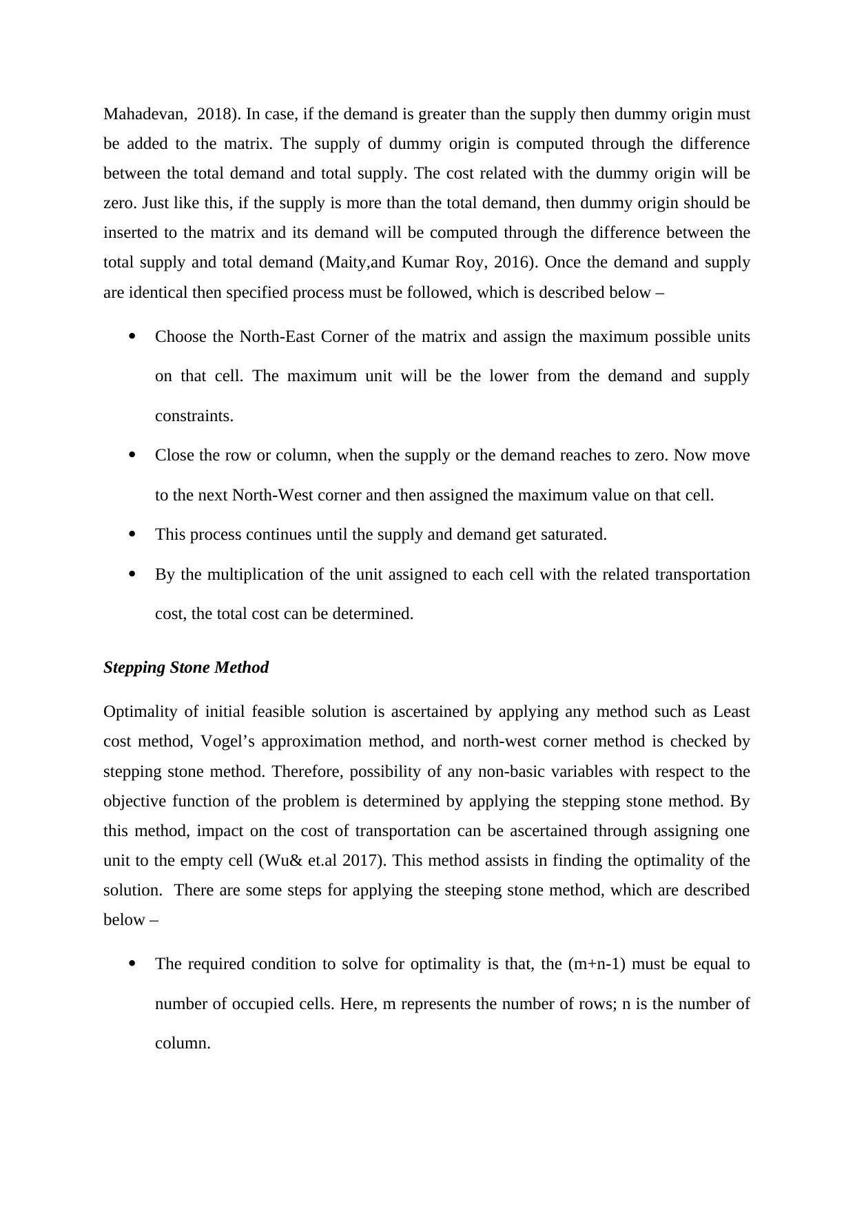
Mahadevan, 2018). In case, if the demand is greater than the supply then dummy origin must
be added to the matrix. The supply of dummy origin is computed through the difference
between the total demand and total supply. The cost related with the dummy origin will be
zero. Just like this, if the supply is more than the total demand, then dummy origin should be
inserted to the matrix and its demand will be computed through the difference between the
total supply and total demand (Maity,and Kumar Roy, 2016). Once the demand and supply
are identical then specified process must be followed, which is described below –
 Choose the North-East Corner of the matrix and assign the maximum possible units
on that cell. The maximum unit will be the lower from the demand and supply
constraints.
 Close the row or column, when the supply or the demand reaches to zero. Now move
to the next North-West corner and then assigned the maximum value on that cell.
 This process continues until the supply and demand get saturated.
 By the multiplication of the unit assigned to each cell with the related transportation
cost, the total cost can be determined.
Stepping Stone Method
Optimality of initial feasible solution is ascertained by applying any method such as Least
cost method, Vogel’s approximation method, and north-west corner method is checked by
stepping stone method. Therefore, possibility of any non-basic variables with respect to the
objective function of the problem is determined by applying the stepping stone method. By
this method, impact on the cost of transportation can be ascertained through assigning one
unit to the empty cell (Wu& et.al 2017). This method assists in finding the optimality of the
solution. There are some steps for applying the steeping stone method, which are described
below –
 The required condition to solve for optimality is that, the (m+n-1) must be equal to
number of occupied cells. Here, m represents the number of rows; n is the number of
column.

 After this, closed loop should be created, by starting it from the unoccupied cell and
return to the same unoccupied cell. This loop can be created by only vertical or
horizontal move.
 After creation of loop, + or – sign assigned to each alternative corner. It is started
from + signs on the unoccupied cell, from where the loop started.
 Until all the unoccupied cells evaluated, these steps should be repeat.
 If all the computed changes are equal to or more than zero, then it is regarded as
optimal solution. However, if it is not, then choose the most negative unoccupied cell
and assign the maximum possible unit. Deduct the unit from the other cells, which has
negative sign in a loop, so that demand and supply requirement can be maintained.
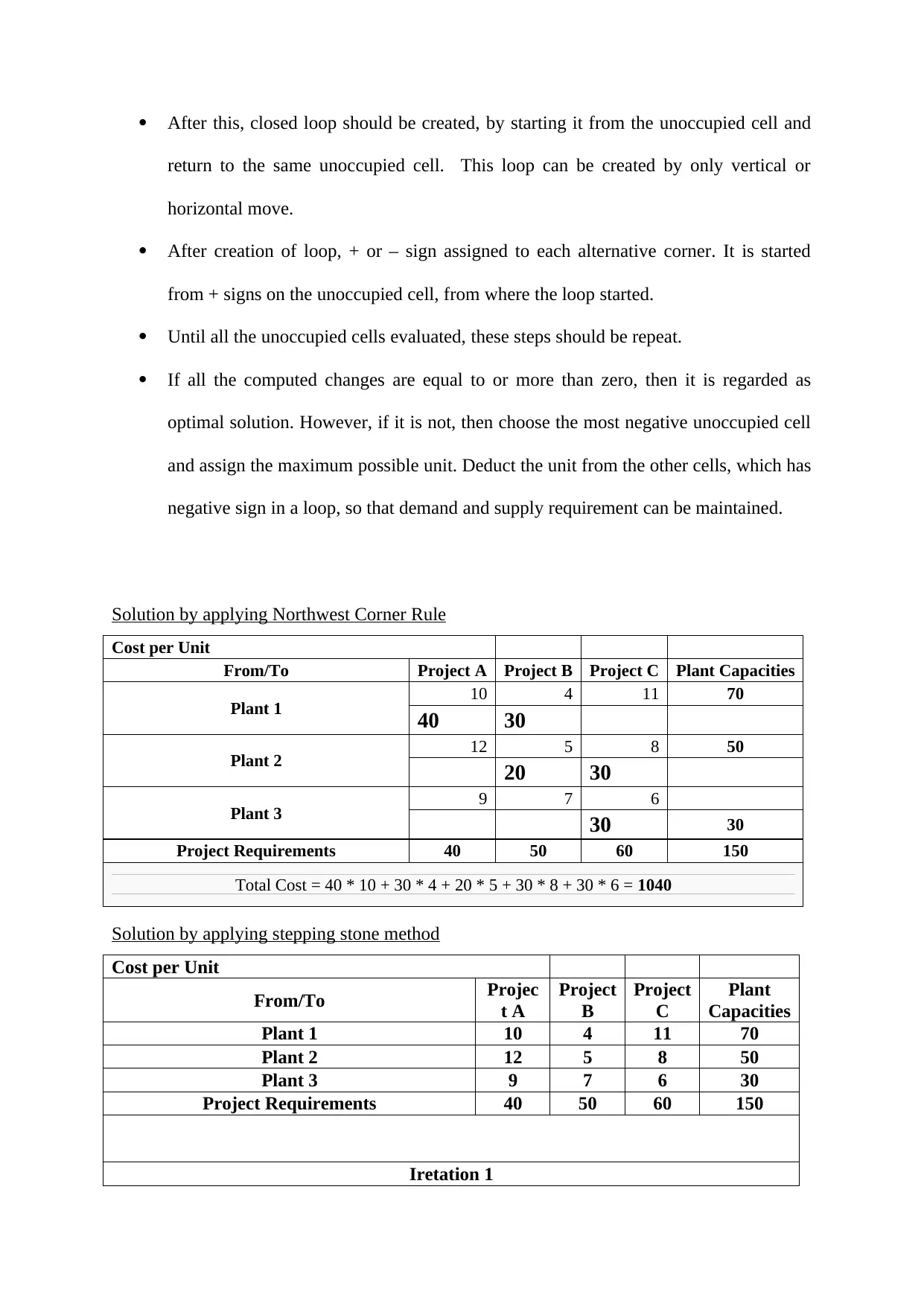
Solution by applying Northwest Corner Rule
Cost per Unit
From/To Project A Project B Project C Plant Capacities
Plant 1 10 4 11 70
40 30
Plant 2 12 5 8 50
20 30
Plant 3 9 7 6
30 30
Project Requirements 40 50 60 150
Total Cost = 40 * 10 + 30 * 4 + 20 * 5 + 30 * 8 + 30 * 6 = 1040
Solution by applying stepping stone method
Cost per Unit
From/To Projec
t A
Project
B
Project
C
Plant
Capacities
Plant 1 10 4 11 70
Plant 2 12 5 8 50
Plant 3 9 7 6 30
Project Requirements 40 50 60 150
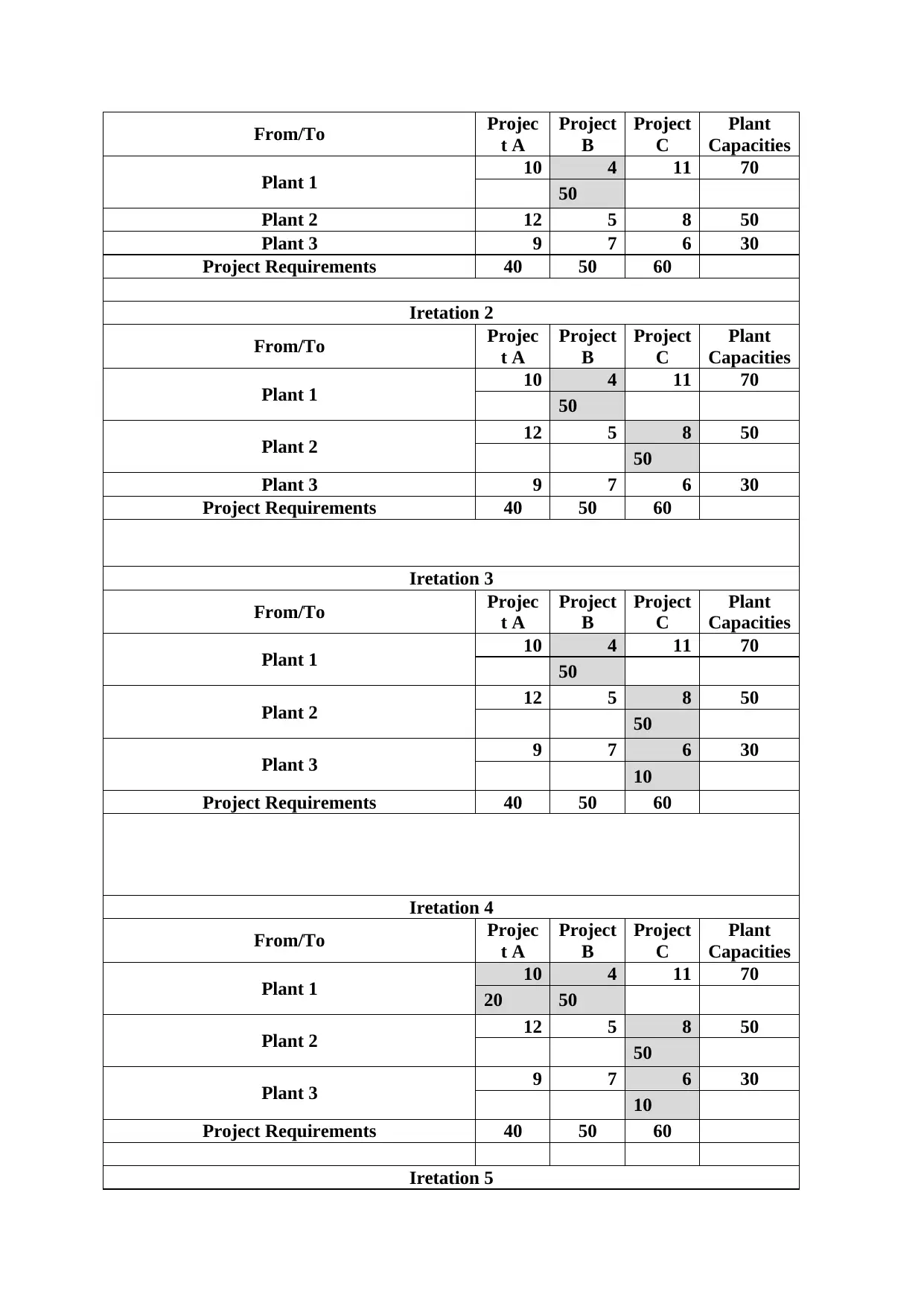
Iretation 1

From/To Projec
t A
Project
B
Project
C
Plant
Capacities
Plant 1 10 4 11 70
50
Plant 2 12 5 8 50
Plant 3 9 7 6 30
Project Requirements 40 50 60
Iretation 2
From/To Projec
t A
Project
B
Project
C
Plant
Capacities
Plant 1 10 4 11 70
50
Plant 2 12 5 8 50
50
Plant 3 9 7 6 30
Project Requirements 40 50 60
Iretation 3
From/To Projec
t A
Project
B
Project
C
Plant
Capacities
Plant 1 10 4 11 70
50
Plant 2 12 5 8 50
50
Plant 3 9 7 6 30
10
Project Requirements 40 50 60
Iretation 4
From/To Projec
t A
Project
B
Project
C
Plant
Capacities
Plant 1 10 4 11 70
20 50
Plant 2 12 5 8 50
50
Plant 3 9 7 6 30
10
Project Requirements 40 50 60
Iretation 5

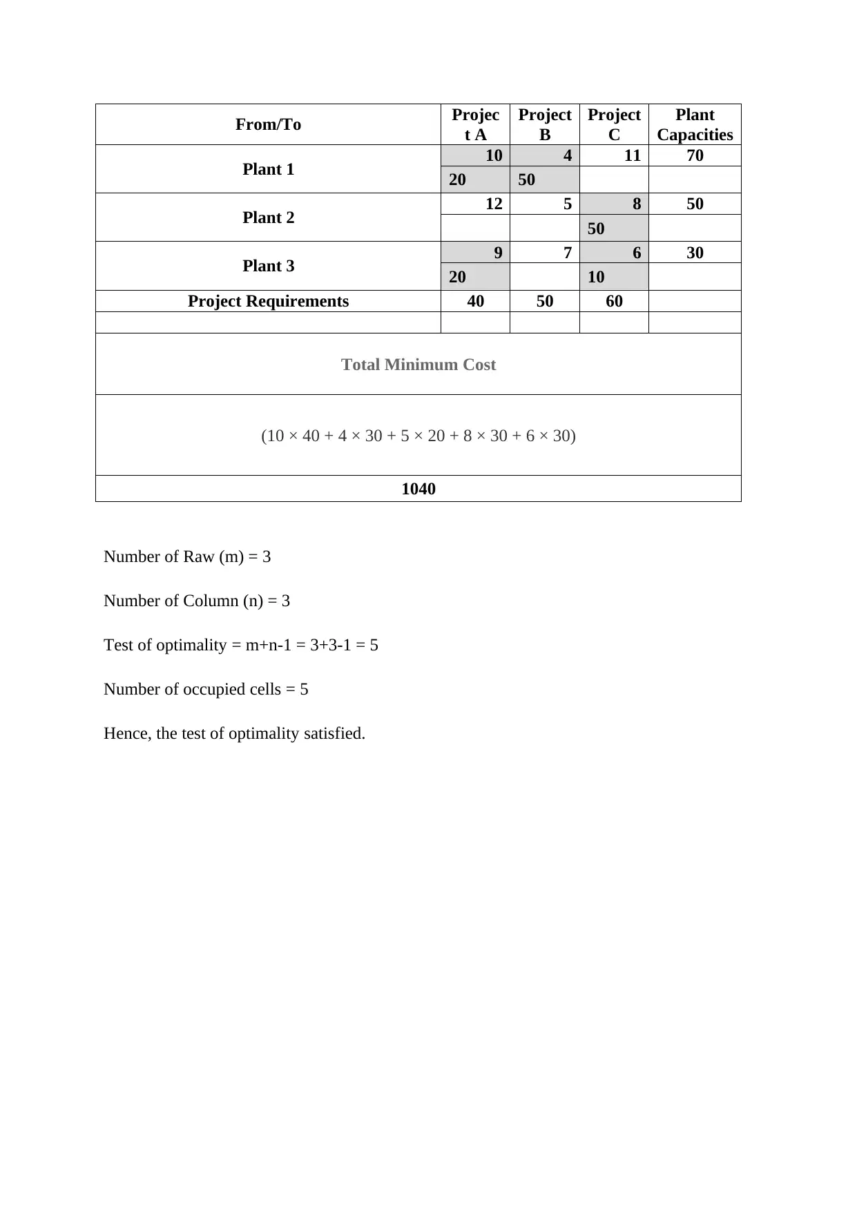
From/To Projec
t A
Project
B
Project
C
Plant
Capacities
Plant 1 10 4 11 70
20 50
Plant 2 12 5 8 50
50
Plant 3 9 7 6 30
20 10
Project Requirements 40 50 60
Total Minimum Cost
(10 × 40 + 4 × 30 + 5 × 20 + 8 × 30 + 6 × 30)
1040
Number of Raw (m) = 3
Number of Column (n) = 3
Test of optimality = m+n-1 = 3+3-1 = 5
Number of occupied cells = 5
Hence, the test of optimality satisfied.

QUESTION 3: DISTRIBUTION AND NETWORK MODEL
The distribution and network model is denoted by a set of arcs, nodes, and function
connected with the nodes or arcs (Zappa, and Lomi, 2015). Many Linear Programming
applications are required to optimize by some types of flows such as goods, resources from
sources to destination. In this model, network is connected by the set of nodes and the nodes
are connected by set of arcs. Decision variables are considered as arcs and constraints are
denoted by nodes (Georgilakis, and Hatziargyriou, 2015).
In the transportation, it is the general problem how to transport goods from set of source to
set of destination by minimum cost.
Nodes
Nodes are the set of source, in which supply is given. Further, it may be set of demand, in
which the demand is given.
Arcs
It is possible routes among the source and destination, having the shipping cost (Newman,
2016).
Objective
The objective of the problem is to determine the route from sources to the destination, by
which the transportation cost can be minimized (Zadorozhnyi, and Yudin, 2015).
In the present study, Moza is the owner of the large camel breeding and company wants to
install a complete water system connecting with several farms. The owner wants to determine
the least expensive way to provide water to each facility. The location and the distance are
given in the problem.

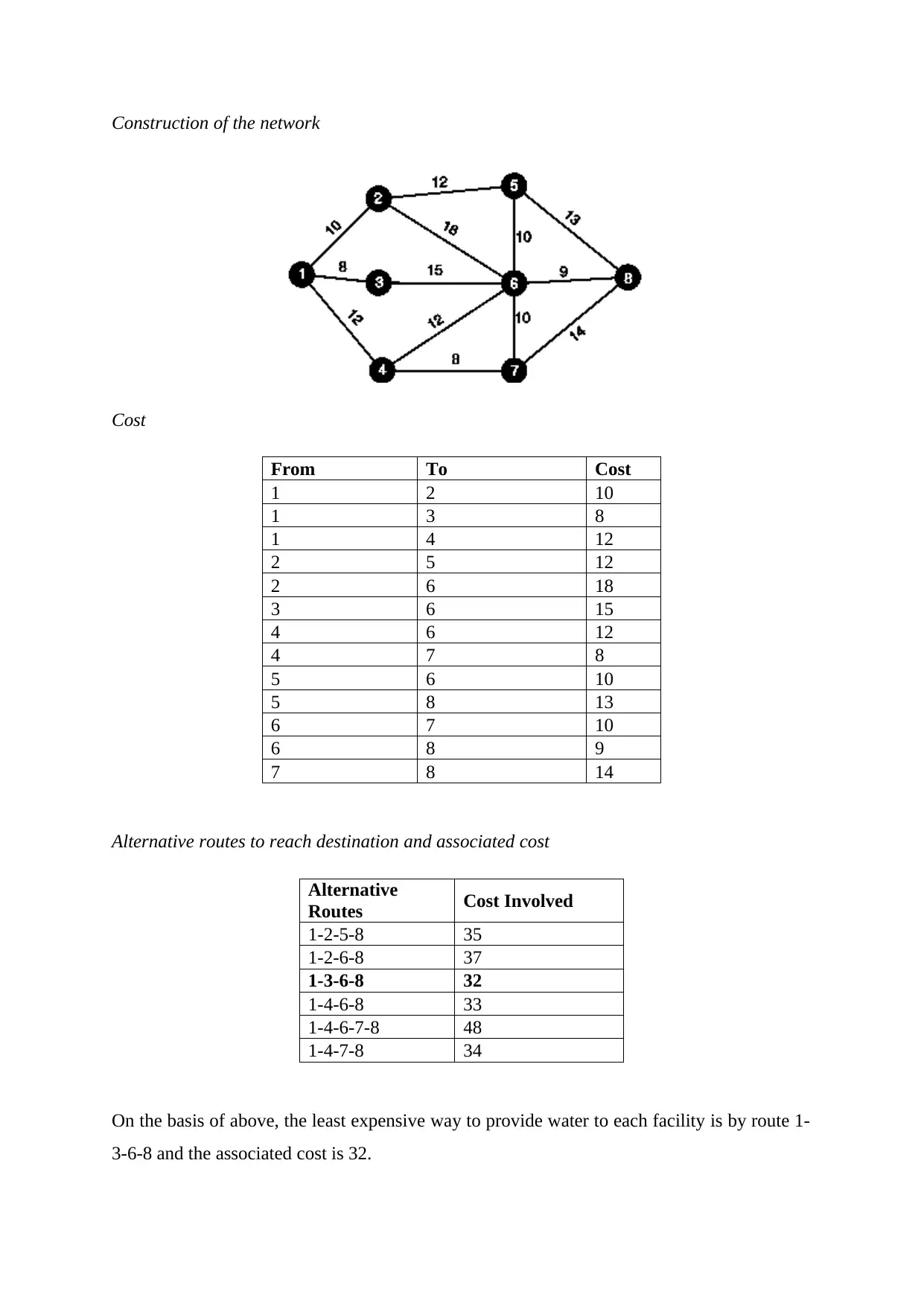
Construction of the network
Cost
From To Cost
1 2 10
1 3 8
1 4 12
2 5 12
2 6 18
3 6 15
4 6 12
4 7 8
5 6 10
5 8 13
6 7 10
6 8 9
7 8 14
Alternative routes to reach destination and associated cost
Alternative
Routes Cost Involved
1-2-5-8 35
1-2-6-8 37
1-3-6-8 32
1-4-6-8 33
1-4-6-7-8 48
1-4-7-8 34
On the basis of above, the least expensive way to provide water to each facility is by route 1-
3-6-8 and the associated cost is 32.

REFERENCES
Bisht, D. and Srivastava, P.K., 2017, October. A unique conversion approach clubbed with a
new ranking technique to optimize fuzzy transportation cost. In AIP Conference
Proceedings (Vol. 1897, No. 1, p. 020023).AIP Publishing.
Dokeroglu, T., 2015.Hybrid teaching–learning-based optimization algorithms for the
Quadratic Assignment Problem. Computers & Industrial Engineering, 85, pp.86-101.
Garrido-Jurado, S., Munoz-Salinas, R., Madrid-Cuevas, F.J. and Medina-Carnicer, R., 2016.
Generation of fiducial marker dictionaries using mixed integer linear programming. Pattern
Recognition, 51, pp.481-491.
Georgilakis, P.S. and Hatziargyriou, N.D., 2015. A review of power distribution planning in
the modern power systems era: Models, methods and future research. Electric Power Systems
Research, 121, pp.89-100.
Gleixner, A.M., Steffy, D.E. and Wolter, K., 2016.Iterative refinement for linear
programming. INFORMS Journal on Computing, 28(3), pp.449-464.
Larsen, C. and Thorstenson, A., 2014. The order and volume fill rates in inventory control
systems. International Journal of Production Economics, 147, pp.13-19.
Ma, D. and Saunders, M.A., 2015.Solving multiscale linear programs using the simplex
method in quadruple precision. In Numerical Analysis and Optimization (pp. 223-235).
Springer, Cham.
Maity, G. and Kumar Roy, S., 2016. Solving a multi-objective transportation problem with
nonlinear cost and multi-choice demand. International Journal of Management Science and
Engineering Management, 11(1), pp.62-70.
METLO, M., SOLANGI, M. and MEMON, S., 2016.Modified North-West Corner Method
for the Optimal Solution for Transportation Problems. Sindh University Research Journal-
SURJ (Science Series), 48(4).
Newman, M.E., 2016. Mathematics of networks. The new Palgrave dictionary of economics,
pp.1-8.

Reyes, J., Solano-Charris, E. and Montoya-Torres, J., 2019. The storage location assignment
problem: A literature review. International Journal of Industrial Engineering
Computations, 10(2), pp.199-224.
Wang, Z.X. and Li, J., 2017. Correlation coefficients of probabilistic hesitant fuzzy elements
and their applications to evaluation of the alternatives. Symmetry, 9(11), p.259.
Wu, P., Chu, F., Che, A. and Fang, Y., 2017.An efficient two-phase exact algorithm for the
automated truck freight transportation problem. Computers & Industrial Engineering, 110,
pp.59-66.
Zadorozhnyi, V.N. and Yudin, E.B., 2015. Growing network: models following nonlinear
preferential attachment rule. Physica A: Statistical Mechanics and its Applications, 428,
pp.111-132.
Zappa, P. and Lomi, A., 2015. The analysis of multilevel networks in organizations: models
and empirical tests. Organizational Research Methods, 18(3), pp.542-569.
Zhang, X. and Mahadevan, S., 2018.A bio-inspired approach to traffic network equilibrium
assignment problem. IEEE transactions on cybernetics, 48(4), pp.1304-1315.