Analysis of Mortar Resistivity: A Civil Engineering Study

This report presents an investigation into the electrical resistivity of conductive mortar, a crucial factor in determining concrete durability. The study examines the relationship between various components of the mortar, including water, cement, sand, and grit, along with environmental factors such as temperature, and the resulting resistivity. The methodology involves data collection, descriptive statistics, correlation analysis, and OLS regression analysis to identify the key factors influencing resistivity. The data, sourced from an existing study, is analyzed to find summary statistics, correlations between variables, and regression models to predict resistivity based on mortar composition. The report discusses the findings, including the significant impact of water and cement content on resistivity, and concludes with insights into the implications of these findings for concrete durability and performance. The analysis also considers the limitations of the data and suggests potential improvements for future studies.

Investigation on the resistivity of conductive mortar
Name
Institution

Table of Contents
Table of Contents..................................................................................................................................2
1. INTRODUCTIONs......................................................................................................................2
2. VARIABLES AND MEASUREMENT......................................................................................3
3. DATA AND METHOD...............................................................................................................4
4. DESCRIPTIVE STATISTICS....................................................................................................5
5. PEARSON’S CORRELATIONS COEFFICIENTS.................................................................6
6. OLS REGRESSION ANALYSIS...............................................................................................9
7. DISCUSSION AND CONCLUSION........................................................................................13
8. References...................................................................................................................................14

Investigation on the Resistivity of Conductive Mortar
1. INTRODUCTION
The durability of concrete refers to the ability of the mortar to withstand any
deterioration process such as abrasion, chemical attach and weathering action and be able to
retain its original serviceability, quality and form when exposed to harsh environment.
Concrete durability is dependent on its ability to resist penetration of aggressive agents [1-3].
The agents may be in liquid or gaseous state and can be transported by several means such as
combination of suction, capillarity, absorption, diffusion and permeation. Therefore, for
concrete already in use, a combined action of these agents may exist through mixed modes of
transport processes [4]. Moreover, there are correlations between electrical conductivity and
the components of mortar (concrete). Other factors that are not considered in this paper that
have correlation with concrete degradation include durability features such as reinforcement
corrosion, chloride ingress, abrasion, acid attack, soft water attack, leaching, frost resistance,
alkali-aggregate reaction, sulphate attack, and carbonation [5-8].
In this paper the transport of ions through concrete microstructure is considered and
analyzed. In case ions are charge in a concrete then it is the duty of the concrete to withstand
the transfer of the ions from one point to the other [9]. This process is highly dependent on
electrical resistivity. Since, components of the mortar are major factors in deterioration of
concrete and plays a role in the electrical resistivity of the concrete [10-14]. When ions are
charged, then it is the concrete’s ability to withstand transfer of charged ions which is highly
dependent upon its electrical resistivity [15]. The components include water, cement, sand
and grit. However, concrete features such as width is also considered in this paper and one
environmental condition (temperature is also recorded).
2. VARIABLES AND MEASUREMENT

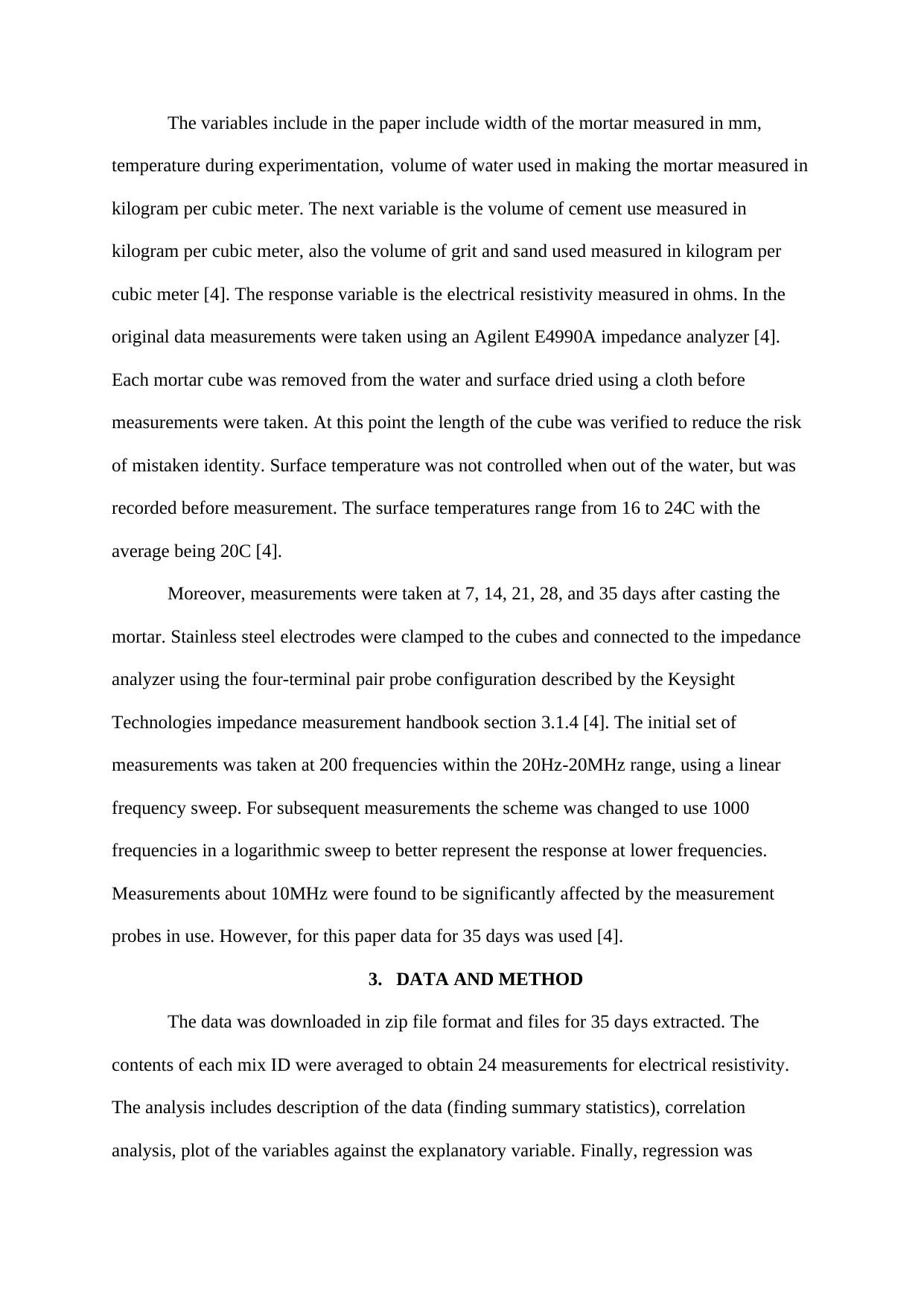
The variables include in the paper include width of the mortar measured in mm,
temperature during experimentation, volume of water used in making the mortar measured in
kilogram per cubic meter. The next variable is the volume of cement use measured in
kilogram per cubic meter, also the volume of grit and sand used measured in kilogram per
cubic meter [4]. The response variable is the electrical resistivity measured in ohms. In the
original data measurements were taken using an Agilent E4990A impedance analyzer [4].
Each mortar cube was removed from the water and surface dried using a cloth before
measurements were taken. At this point the length of the cube was verified to reduce the risk
of mistaken identity. Surface temperature was not controlled when out of the water, but was
recorded before measurement. The surface temperatures range from 16 to 24C with the
average being 20C [4].
Moreover, measurements were taken at 7, 14, 21, 28, and 35 days after casting the
mortar. Stainless steel electrodes were clamped to the cubes and connected to the impedance
analyzer using the four-terminal pair probe configuration described by the Keysight
Technologies impedance measurement handbook section 3.1.4 [4]. The initial set of
measurements was taken at 200 frequencies within the 20Hz-20MHz range, using a linear
frequency sweep. For subsequent measurements the scheme was changed to use 1000
frequencies in a logarithmic sweep to better represent the response at lower frequencies.
Measurements about 10MHz were found to be significantly affected by the measurement
probes in use. However, for this paper data for 35 days was used [4].
3. DATA AND METHOD
The data was downloaded in zip file format and files for 35 days extracted. The
contents of each mix ID were averaged to obtain 24 measurements for electrical resistivity.
The analysis includes description of the data (finding summary statistics), correlation
analysis, plot of the variables against the explanatory variable. Finally, regression was

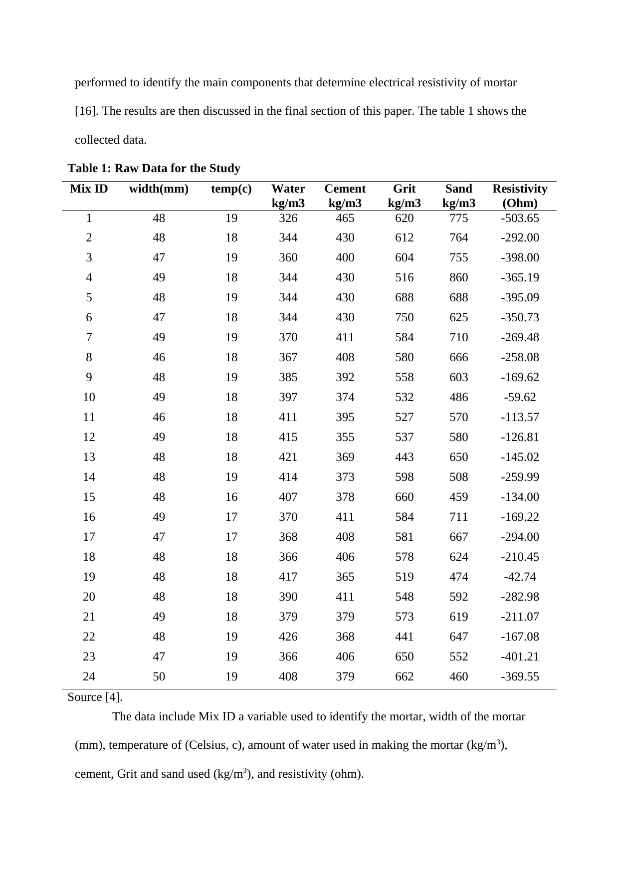
performed to identify the main components that determine electrical resistivity of mortar
[16]. The results are then discussed in the final section of this paper. The table 1 shows the
collected data.
Table 1: Raw Data for the Study
Mix ID width(mm) temp(c) Water
kg/m3
Cement
kg/m3
Grit
kg/m3
Sand
kg/m3
Resistivity
(Ohm)
1 48 19 326 465 620 775 -503.65
2 48 18 344 430 612 764 -292.00
3 47 19 360 400 604 755 -398.00
4 49 18 344 430 516 860 -365.19
5 48 19 344 430 688 688 -395.09
6 47 18 344 430 750 625 -350.73
7 49 19 370 411 584 710 -269.48
8 46 18 367 408 580 666 -258.08
9 48 19 385 392 558 603 -169.62
10 49 18 397 374 532 486 -59.62
11 46 18 411 395 527 570 -113.57
12 49 18 415 355 537 580 -126.81
13 48 18 421 369 443 650 -145.02
14 48 19 414 373 598 508 -259.99
15 48 16 407 378 660 459 -134.00
16 49 17 370 411 584 711 -169.22
17 47 17 368 408 581 667 -294.00
18 48 18 366 406 578 624 -210.45
19 48 18 417 365 519 474 -42.74
20 48 18 390 411 548 592 -282.98
21 49 18 379 379 573 619 -211.07
22 48 19 426 368 441 647 -167.08
23 47 19 366 406 650 552 -401.21
24 50 19 408 379 662 460 -369.55
Source [4].
The data include Mix ID a variable used to identify the mortar, width of the mortar
(mm), temperature of (Celsius, c), amount of water used in making the mortar (kg/m3),
cement, Grit and sand used (kg/m3), and resistivity (ohm).

4. DESCRIPTIVE STATISTICS
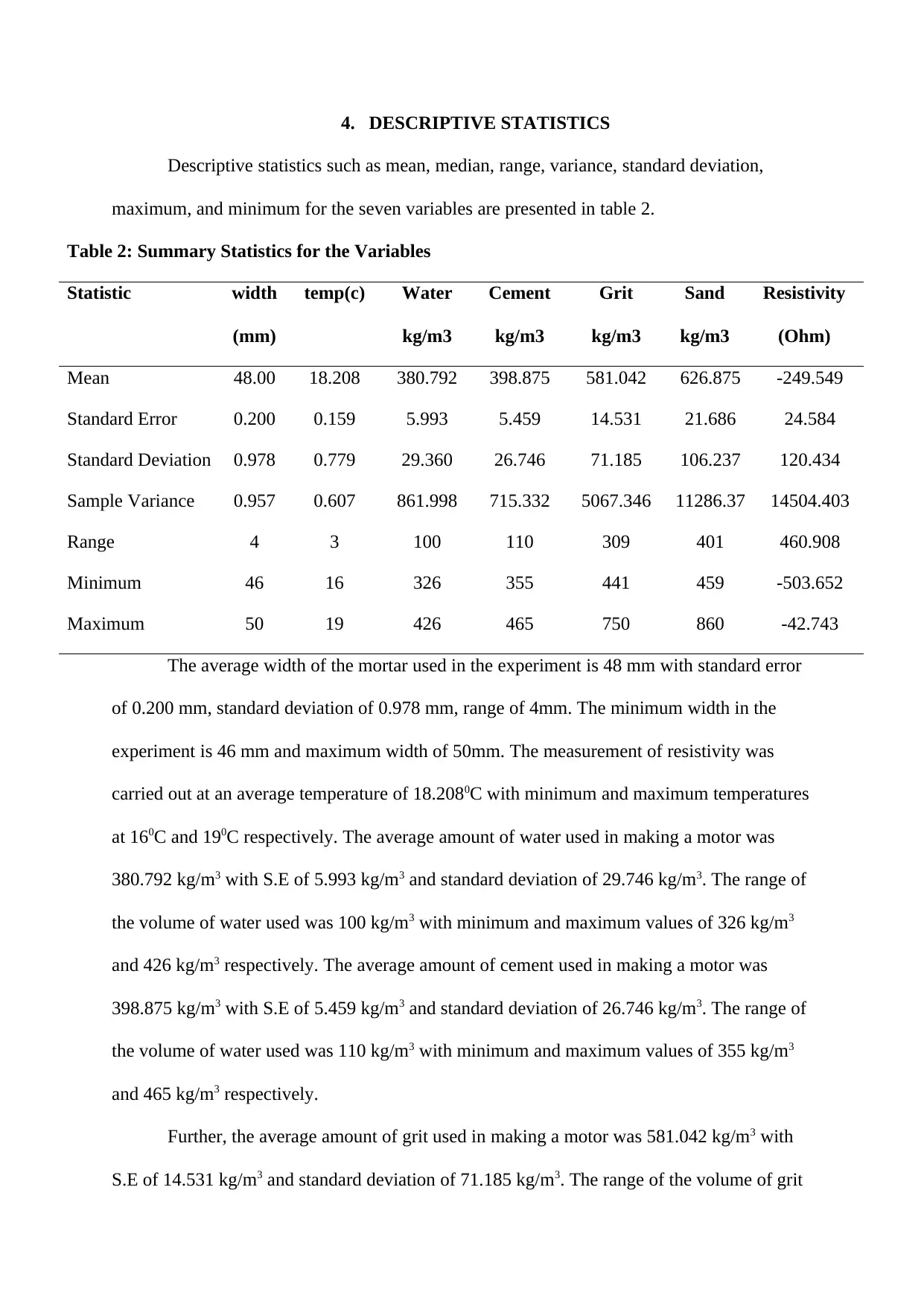
Descriptive statistics such as mean, median, range, variance, standard deviation,
maximum, and minimum for the seven variables are presented in table 2.
Table 2: Summary Statistics for the Variables
Statistic width
(mm)
temp(c) Water
kg/m3
Cement
kg/m3
Grit
kg/m3
Sand
kg/m3
Resistivity
(Ohm)
Mean 48.00 18.208 380.792 398.875 581.042 626.875 -249.549
Standard Error 0.200 0.159 5.993 5.459 14.531 21.686 24.584
Standard Deviation 0.978 0.779 29.360 26.746 71.185 106.237 120.434
Sample Variance 0.957 0.607 861.998 715.332 5067.346 11286.37 14504.403
Range 4 3 100 110 309 401 460.908
Minimum 46 16 326 355 441 459 -503.652
Maximum 50 19 426 465 750 860 -42.743
The average width of the mortar used in the experiment is 48 mm with standard error
of 0.200 mm, standard deviation of 0.978 mm, range of 4mm. The minimum width in the
experiment is 46 mm and maximum width of 50mm. The measurement of resistivity was
carried out at an average temperature of 18.2080C with minimum and maximum temperatures
at 160C and 190C respectively. The average amount of water used in making a motor was
380.792 kg/m3 with S.E of 5.993 kg/m3 and standard deviation of 29.746 kg/m3. The range of
the volume of water used was 100 kg/m3 with minimum and maximum values of 326 kg/m3
and 426 kg/m3 respectively. The average amount of cement used in making a motor was
398.875 kg/m3 with S.E of 5.459 kg/m3 and standard deviation of 26.746 kg/m3. The range of
the volume of water used was 110 kg/m3 with minimum and maximum values of 355 kg/m3
and 465 kg/m3 respectively.
Further, the average amount of grit used in making a motor was 581.042 kg/m3 with
S.E of 14.531 kg/m3 and standard deviation of 71.185 kg/m3. The range of the volume of grit

used was 309 kg/m3 with minimum and maximum values of 441 kg/m3 and 750 kg/m3
respectively. The average amount of sand used in making a motor was 626.875 kg/m3 with
S.E of 21.686 kg/m3 and standard deviation of 106.237 kg/m3. The range of the volume of
water used was 401 kg/m3 with minimum and maximum values of 459 kg/m3 and 860 kg/m3
respectively. Finally, the measured resistance had an average value of -249.549Ω S.E of
24.584 Ω and standard deviation of 120.434 Ω. The range of the resistivity is 460.908 Ω with
minimum and maximum values of -503.652 Ω and -42.743 Ω.
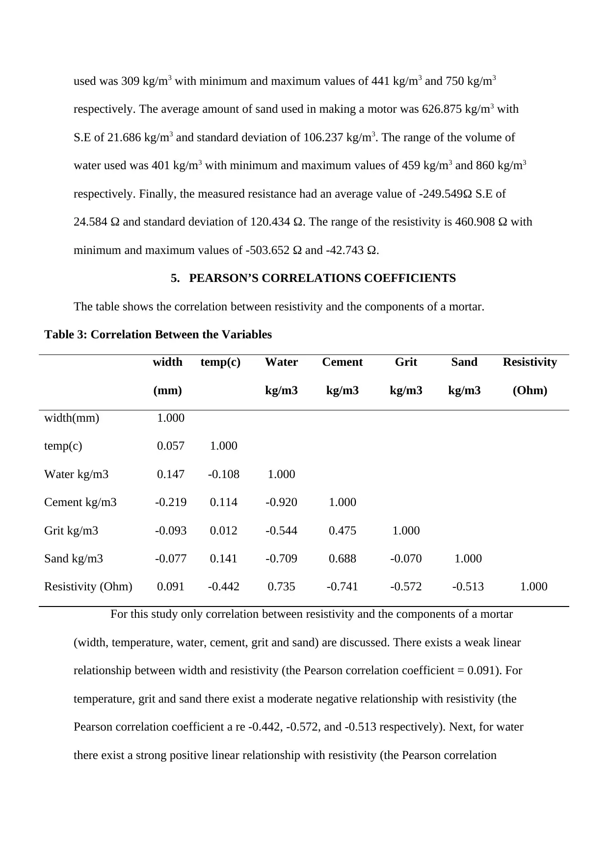
5. PEARSON’S CORRELATIONS COEFFICIENTS
The table shows the correlation between resistivity and the components of a mortar.
Table 3: Correlation Between the Variables
width
(mm)
temp(c) Water
kg/m3
Cement
kg/m3
Grit
kg/m3
Sand
kg/m3
Resistivity
(Ohm)
width(mm) 1.000
temp(c) 0.057 1.000
Water kg/m3 0.147 -0.108 1.000
Cement kg/m3 -0.219 0.114 -0.920 1.000
Grit kg/m3 -0.093 0.012 -0.544 0.475 1.000
Sand kg/m3 -0.077 0.141 -0.709 0.688 -0.070 1.000
Resistivity (Ohm) 0.091 -0.442 0.735 -0.741 -0.572 -0.513 1.000
For this study only correlation between resistivity and the components of a mortar
(width, temperature, water, cement, grit and sand) are discussed. There exists a weak linear
relationship between width and resistivity (the Pearson correlation coefficient = 0.091). For
temperature, grit and sand there exist a moderate negative relationship with resistivity (the
Pearson correlation coefficient a re -0.442, -0.572, and -0.513 respectively). Next, for water
there exist a strong positive linear relationship with resistivity (the Pearson correlation

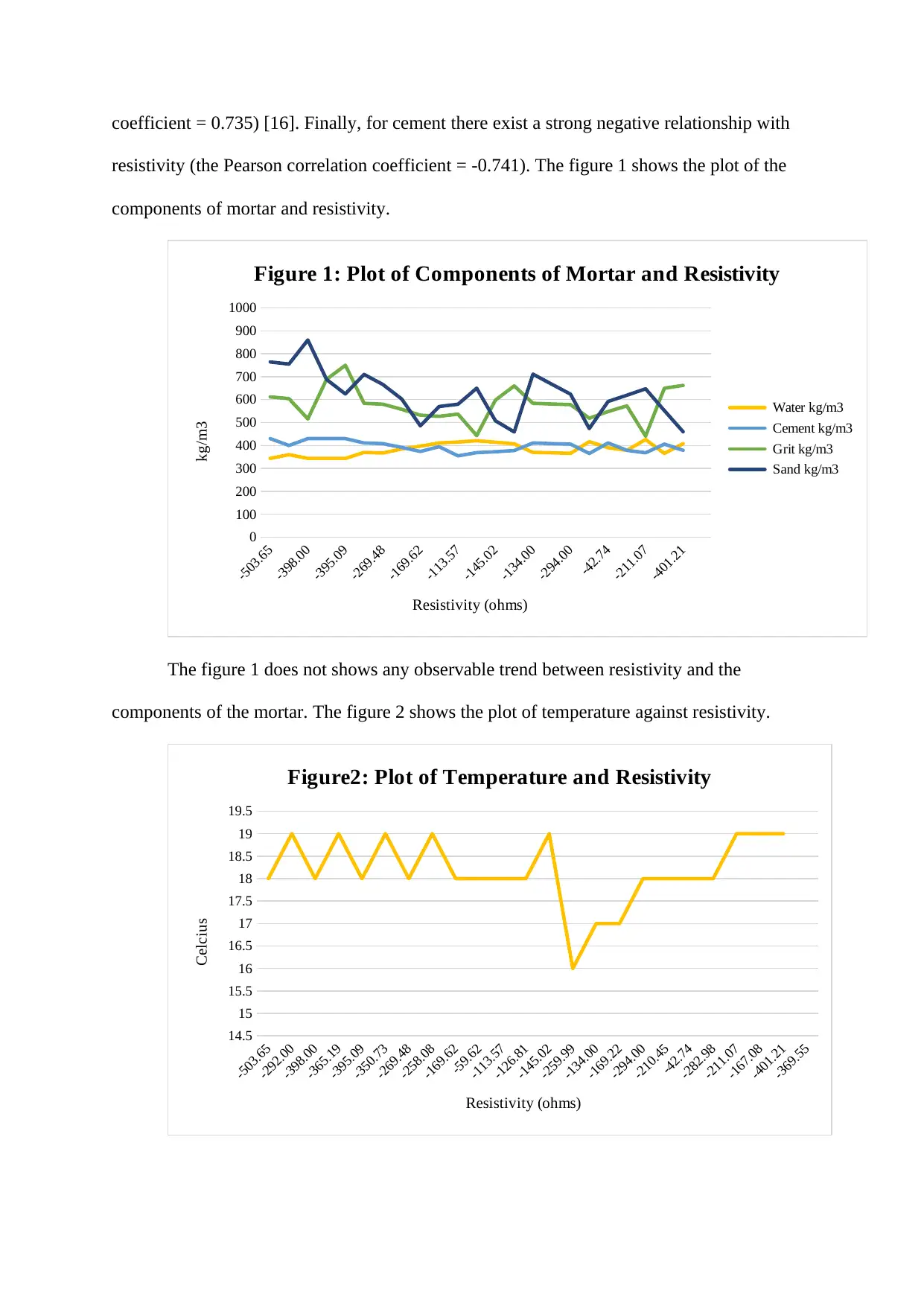
coefficient = 0.735) [16]. Finally, for cement there exist a strong negative relationship with
resistivity (the Pearson correlation coefficient = -0.741). The figure 1 shows the plot of the
components of mortar and resistivity.
-503.65
-398.00
-395.09
-269.48
-169.62
-113.57
-145.02
-134.00
-294.00
-42.74
-211.07
-401.21
0
100
200
300
400
500
600
700
800
900
1000
Figure 1: Plot of Components of Mortar and Resistivity
Water kg/m3
Cement kg/m3
Grit kg/m3
Sand kg/m3
Resistivity (ohms)
kg/m3
The figure 1 does not shows any observable trend between resistivity and the
components of the mortar. The figure 2 shows the plot of temperature against resistivity.
-503.65
-292.00
-398.00
-365.19
-395.09
-350.73
-269.48
-258.08
-169.62
-59.62
-113.57
-126.81
-145.02
-259.99
-134.00
-169.22
-294.00
-210.45
-42.74
-282.98
-211.07
-167.08
-401.21
-369.55
14.5
15
15.5
16
16.5
17
17.5
18
18.5
19
19.5
Figure2: Plot of Temperature and Resistivity
Resistivity (ohms)
Celcius

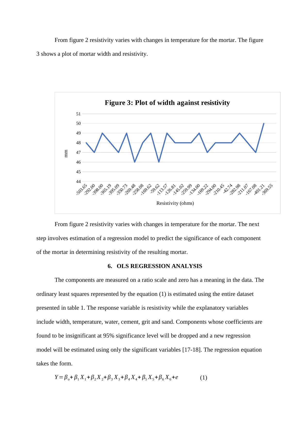
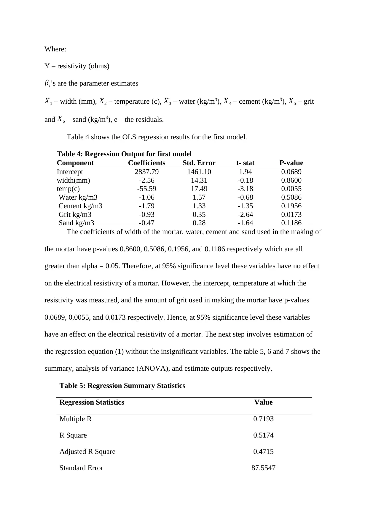
From figure 2 resistivity varies with changes in temperature for the mortar. The figure
3 shows a plot of mortar width and resistivity.
-503.65
-292.00
-398.00
-365.19
-395.09
-350.73
-269.48
-258.08
-169.62
-59.62
-113.57
-126.81
-145.02
-259.99
-134.00
-169.22
-294.00
-210.45
-42.74
-282.98
-211.07
-167.08
-401.21
-369.55
44
45
46
47
48
49
50
51
Figure 3: Plot of width against resistivity
Resistivity (ohms)
mm
From figure 2 resistivity varies with changes in temperature for the mortar. The next
step involves estimation of a regression model to predict the significance of each component
of the mortar in determining resistivity of the resulting mortar.
6. OLS REGRESSION ANALYSIS
The components are measured on a ratio scale and zero has a meaning in the data. The
ordinary least squares represented by the equation (1) is estimated using the entire dataset
presented in table 1. The response variable is resistivity while the explanatory variables
include width, temperature, water, cement, grit and sand. Components whose coefficients are
found to be insignificant at 95% significance level will be dropped and a new regression
model will be estimated using only the significant variables [17-18]. The regression equation
takes the form.
Y = βo+ β1 X1 +β2 X 2+ β3 X3 + β4 X4 + β5 X5 +β6 X6 +e (1)

Where:
Y – resistivity (ohms)
βi’s are the parameter estimates
X1 – width (mm), X2 – temperature (c), X3 – water (kg/m3), X 4 – cement (kg/m3), X5 – grit
and X6 – sand (kg/m3), e – the residuals.
Table 4 shows the OLS regression results for the first model.
Table 4: Regression Output for first model
Component Coefficients Std. Error t- stat P-value
Intercept 2837.79 1461.10 1.94 0.0689
width(mm) -2.56 14.31 -0.18 0.8600
temp(c) -55.59 17.49 -3.18 0.0055
Water kg/m3 -1.06 1.57 -0.68 0.5086
Cement kg/m3 -1.79 1.33 -1.35 0.1956
Grit kg/m3 -0.93 0.35 -2.64 0.0173
Sand kg/m3 -0.47 0.28 -1.64 0.1186
The coefficients of width of the mortar, water, cement and sand used in the making of
the mortar have p-values 0.8600, 0.5086, 0.1956, and 0.1186 respectively which are all
greater than alpha = 0.05. Therefore, at 95% significance level these variables have no effect
on the electrical resistivity of a mortar. However, the intercept, temperature at which the
resistivity was measured, and the amount of grit used in making the mortar have p-values
0.0689, 0.0055, and 0.0173 respectively. Hence, at 95% significance level these variables
have an effect on the electrical resistivity of a mortar. The next step involves estimation of
the regression equation (1) without the insignificant variables. The table 5, 6 and 7 shows the
summary, analysis of variance (ANOVA), and estimate outputs respectively.
Table 5: Regression Summary Statistics
Regression Statistics Value
Multiple R 0.7193
R Square 0.5174
Adjusted R Square 0.4715
Standard Error 87.5547

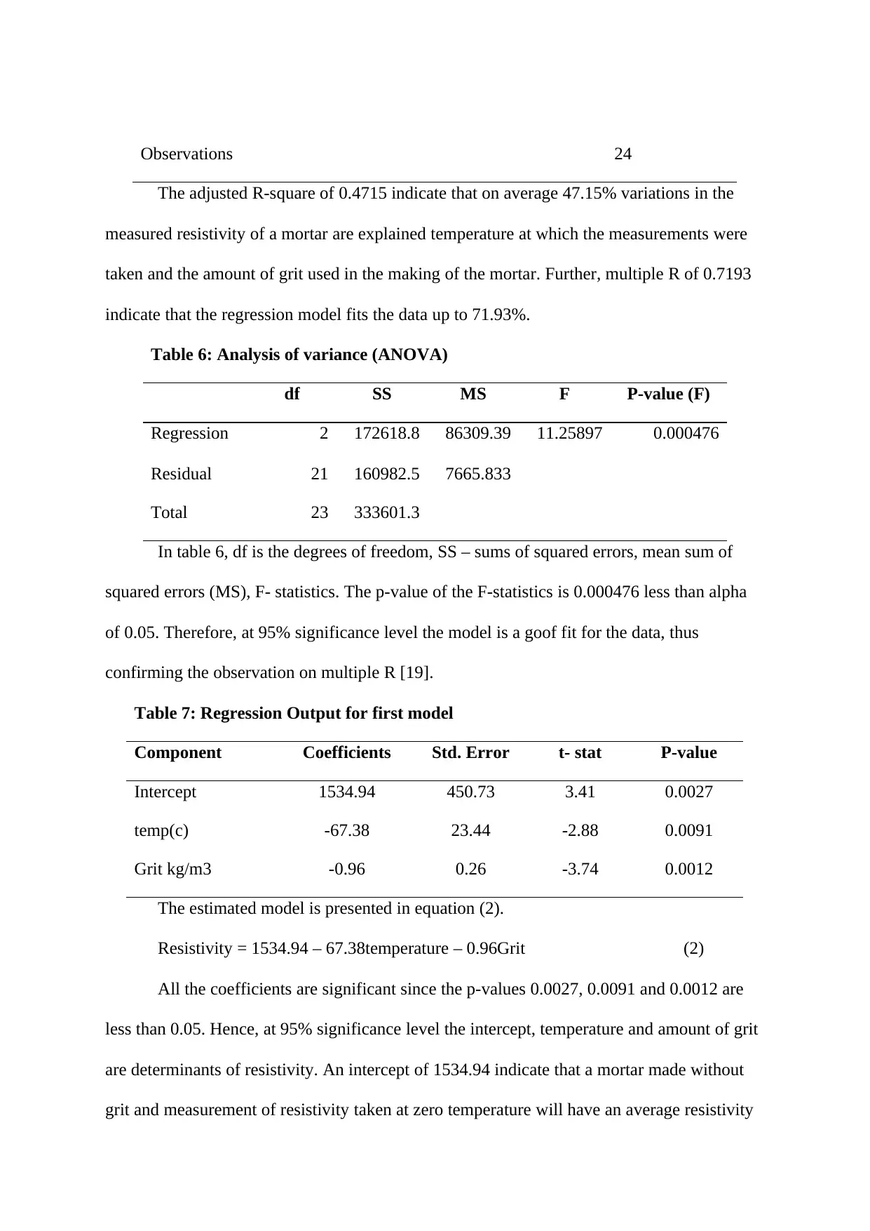
Observations 24
The adjusted R-square of 0.4715 indicate that on average 47.15% variations in the
measured resistivity of a mortar are explained temperature at which the measurements were
taken and the amount of grit used in the making of the mortar. Further, multiple R of 0.7193
indicate that the regression model fits the data up to 71.93%.
Table 6: Analysis of variance (ANOVA)
df SS MS F P-value (F)
Regression 2 172618.8 86309.39 11.25897 0.000476
Residual 21 160982.5 7665.833
Total 23 333601.3
In table 6, df is the degrees of freedom, SS – sums of squared errors, mean sum of
squared errors (MS), F- statistics. The p-value of the F-statistics is 0.000476 less than alpha
of 0.05. Therefore, at 95% significance level the model is a goof fit for the data, thus
confirming the observation on multiple R [19].
Table 7: Regression Output for first model
Component Coefficients Std. Error t- stat P-value
Intercept 1534.94 450.73 3.41 0.0027
temp(c) -67.38 23.44 -2.88 0.0091
Grit kg/m3 -0.96 0.26 -3.74 0.0012
The estimated model is presented in equation (2).
Resistivity = 1534.94 – 67.38temperature – 0.96Grit (2)
All the coefficients are significant since the p-values 0.0027, 0.0091 and 0.0012 are
less than 0.05. Hence, at 95% significance level the intercept, temperature and amount of grit
are determinants of resistivity. An intercept of 1534.94 indicate that a mortar made without
grit and measurement of resistivity taken at zero temperature will have an average resistivity

of 1534.94Ω. Coefficient of temperature of -67.38 indicate that a unit change in temperature
at which the measurements of resistivity is taken on average cause a decline in resistivity by
67.38 Ω. Finally, the coefficient of grit of -0.96 indicate that increasing the volume of grit by
1 kg/m3 while making a mortar on average reduce resistivity by 0.96 Ω. However, the results
of the regression are not useful if the assumptions of the multiple OLS are not met. The
assumptions include (1) linearity between responses and explanatory variables, (2) normality
of the residuals, (3) independence and (4) homoscedasticity (constant variance) [20].
The linearity assumption is met as shown in table 3, there exist a linear relationship
between temperature and grit with resistivity. The second assumption is diagnosed with
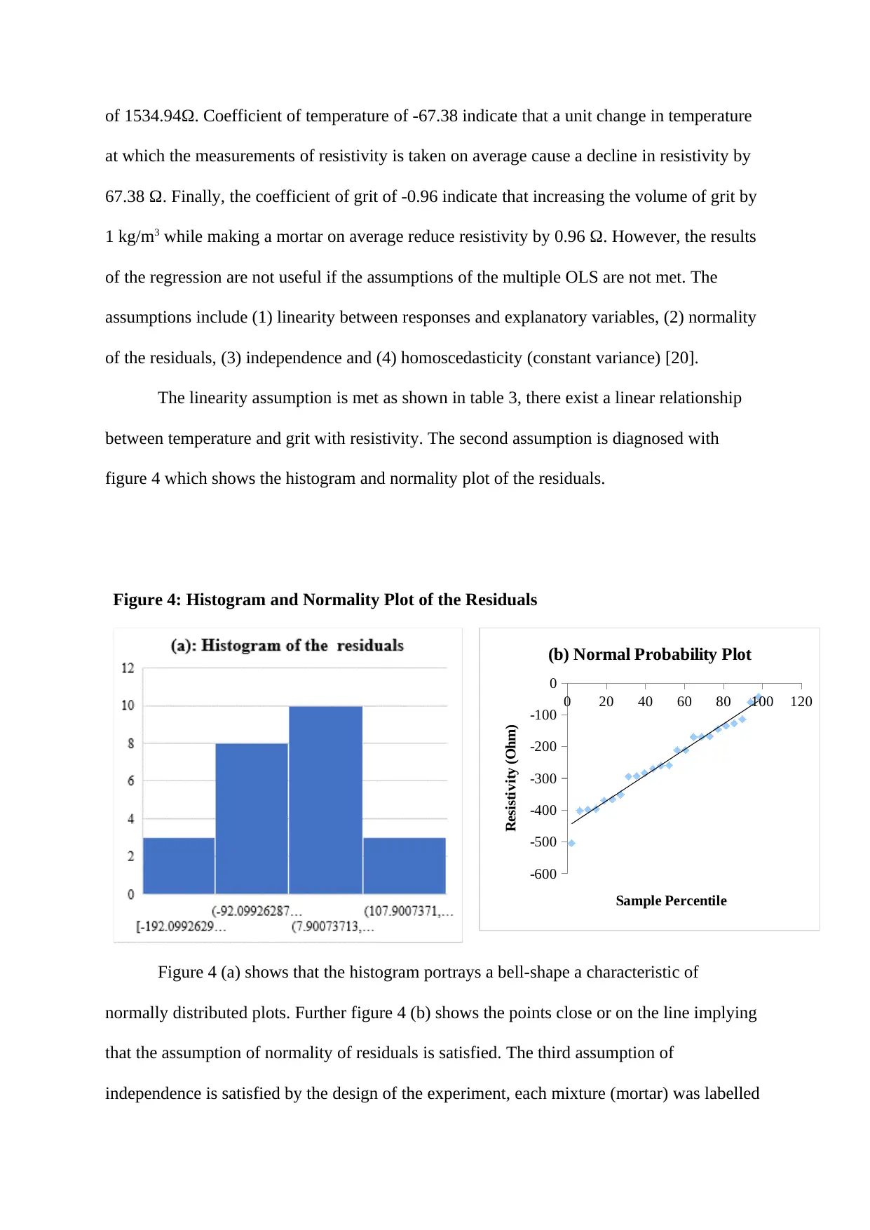
figure 4 which shows the histogram and normality plot of the residuals.
Figure 4: Histogram and Normality Plot of the Residuals
0 20 40 60 80 100 120
-600
-500
-400
-300
-200
-100
0
(b) Normal Probability Plot
Sample Percentile
Resistivity (Ohm)
Figure 4 (a) shows that the histogram portrays a bell-shape a characteristic of
normally distributed plots. Further figure 4 (b) shows the points close or on the line implying
that the assumption of normality of residuals is satisfied. The third assumption of
independence is satisfied by the design of the experiment, each mixture (mortar) was labelled