Financial Distress Analysis of Companies

The assignment delves into the analysis of financial distress prediction using key financial ratios. It explores ratios like profit margin, return on assets, total debt to equity ratio, current ratio, quick ratio, and total costs/total sales ratio. The focus is on comparing these ratios between bankrupt and non-bankrupt companies to identify significant differences indicative of potential financial distress. Statistical tests are employed to assess the significance of these differences, aiding in understanding which ratios are most effective predictors of bankruptcy.

Running head: DATA ANALYSIS ASSIGNMENT
Data Analysis Assignment
Name
Course Number
Date
Faculty Name

DATA ANALYSIS ASSIGNMENT 2
Question 1
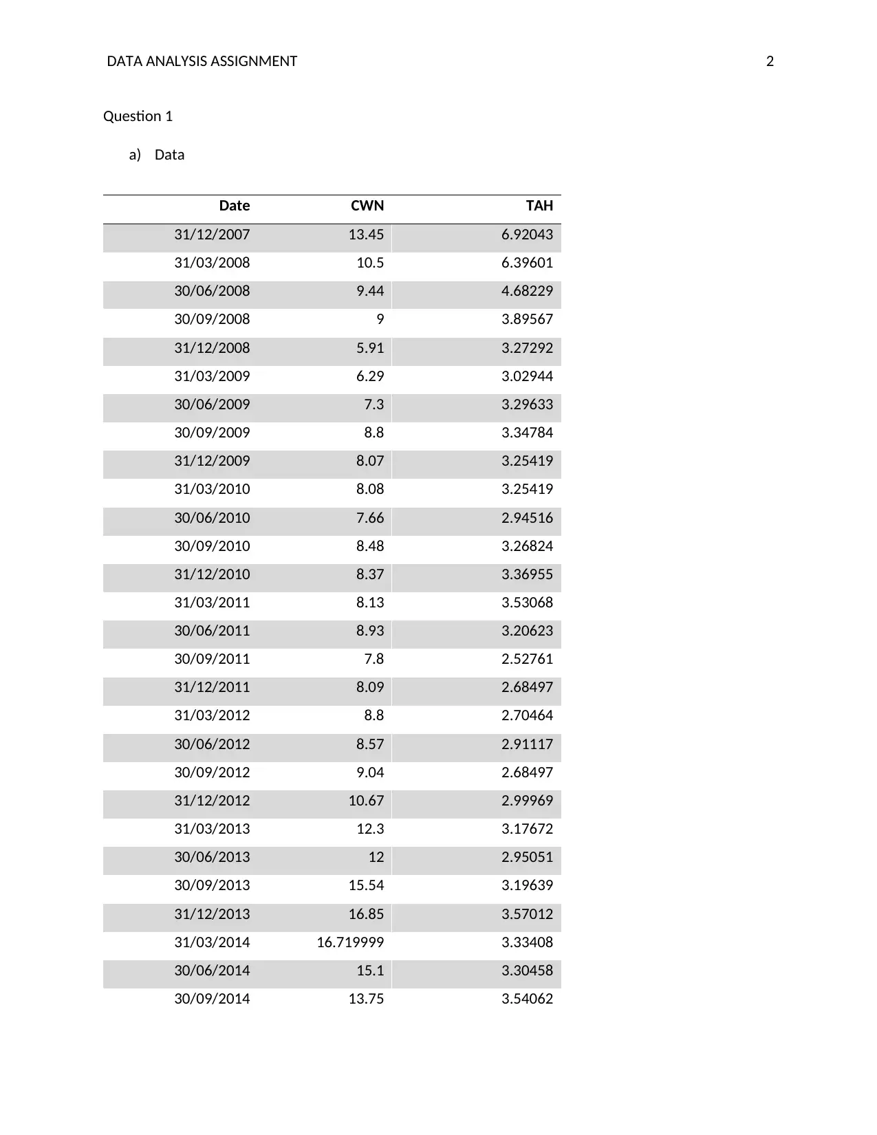
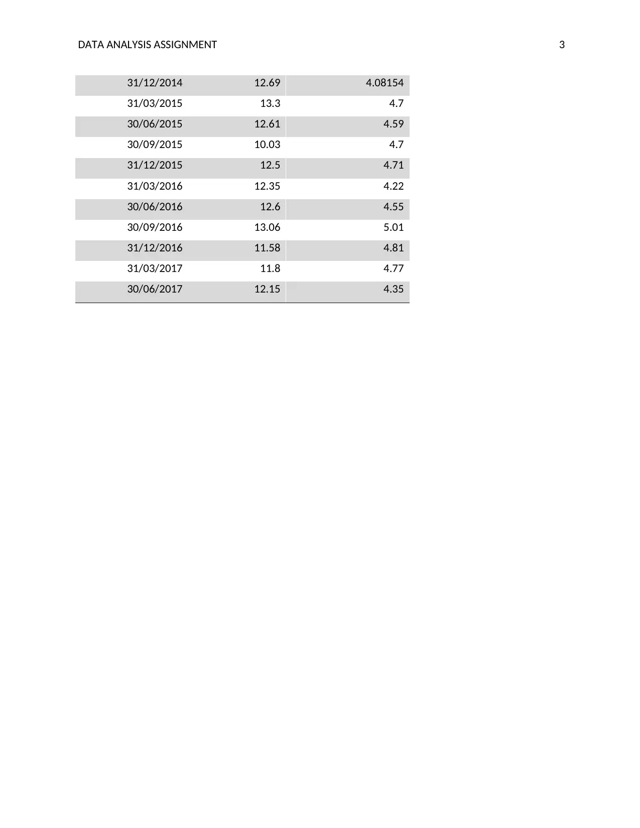
a) Data
Date CWN TAH
31/12/2007 13.45 6.92043
31/03/2008 10.5 6.39601
30/06/2008 9.44 4.68229
30/09/2008 9 3.89567
31/12/2008 5.91 3.27292
31/03/2009 6.29 3.02944
30/06/2009 7.3 3.29633
30/09/2009 8.8 3.34784
31/12/2009 8.07 3.25419
31/03/2010 8.08 3.25419
30/06/2010 7.66 2.94516
30/09/2010 8.48 3.26824
31/12/2010 8.37 3.36955
31/03/2011 8.13 3.53068
30/06/2011 8.93 3.20623
30/09/2011 7.8 2.52761
31/12/2011 8.09 2.68497
31/03/2012 8.8 2.70464
30/06/2012 8.57 2.91117
30/09/2012 9.04 2.68497
31/12/2012 10.67 2.99969
31/03/2013 12.3 3.17672
30/06/2013 12 2.95051
30/09/2013 15.54 3.19639
31/12/2013 16.85 3.57012
31/03/2014 16.719999 3.33408
30/06/2014 15.1 3.30458
30/09/2014 13.75 3.54062

DATA ANALYSIS ASSIGNMENT 3
31/12/2014 12.69 4.08154
31/03/2015 13.3 4.7
30/06/2015 12.61 4.59
30/09/2015 10.03 4.7
31/12/2015 12.5 4.71
31/03/2016 12.35 4.22
30/06/2016 12.6 4.55
30/09/2016 13.06 5.01
31/12/2016 11.58 4.81
31/03/2017 11.8 4.77
30/06/2017 12.15 4.35

DATA ANALYSIS ASSIGNMENT 4
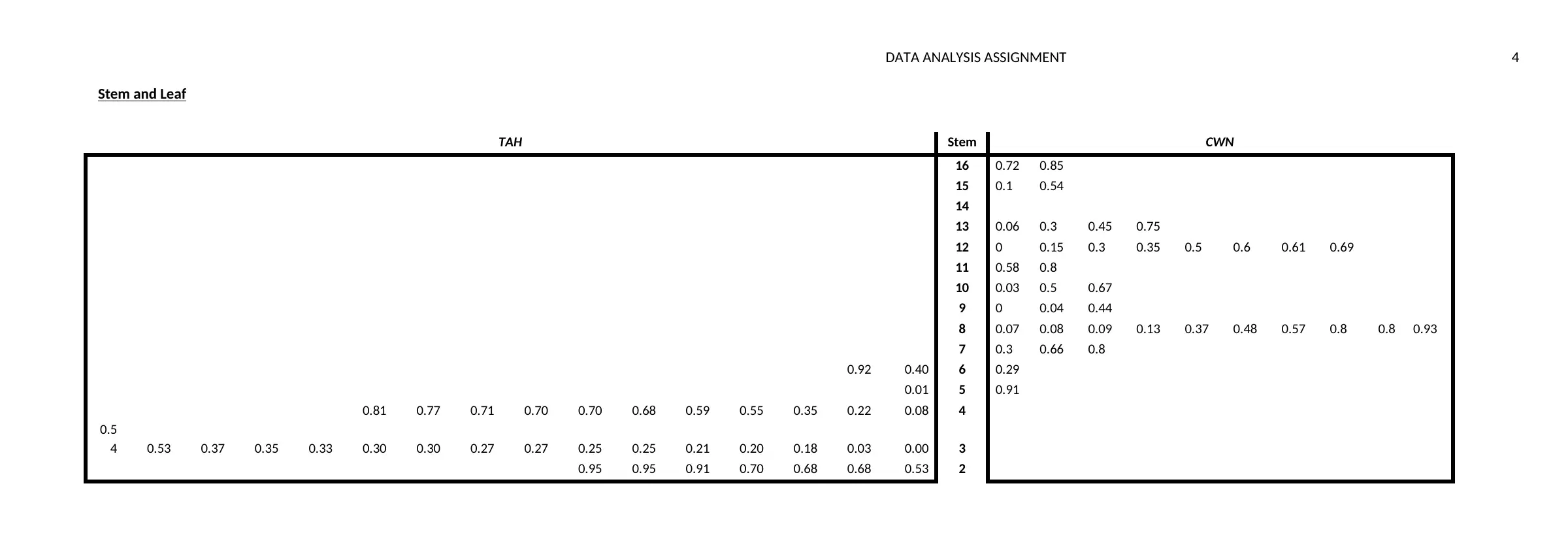
Stem and Leaf
TAH Stem CWN
16 0.72 0.85
15 0.1 0.54
14
13 0.06 0.3 0.45 0.75
12 0 0.15 0.3 0.35 0.5 0.6 0.61 0.69
11 0.58 0.8
10 0.03 0.5 0.67
9 0 0.04 0.44
8 0.07 0.08 0.09 0.13 0.37 0.48 0.57 0.8 0.8 0.93
7 0.3 0.66 0.8
0.92 0.40 6 0.29
0.01 5 0.91
0.81 0.77 0.71 0.70 0.70 0.68 0.59 0.55 0.35 0.22 0.08 4
0.5
4 0.53 0.37 0.35 0.33 0.30 0.30 0.27 0.27 0.25 0.25 0.21 0.20 0.18 0.03 0.00 3
0.95 0.95 0.91 0.70 0.68 0.68 0.53 2

DATA ANALYSIS ASSIGNMENT 5
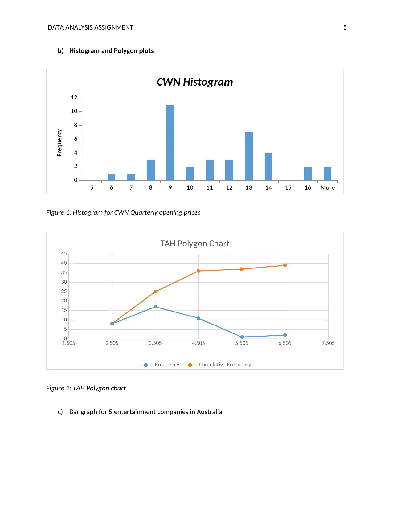
b) Histogram and Polygon plots
5 6 7 8 9 10 11 12 13 14 15 16 More
0
2
4
6
8
10
12
CWN Histogram
Frequency
Figure 1: Histogram for CWN Quarterly opening prices
1.505 2.505 3.505 4.505 5.505 6.505 7.505
0
5
10
15
20
25
30
35
40
45
TAH Polygon Chart
Frequency Cumulative Frequency
Figure 2: TAH Polygon chart
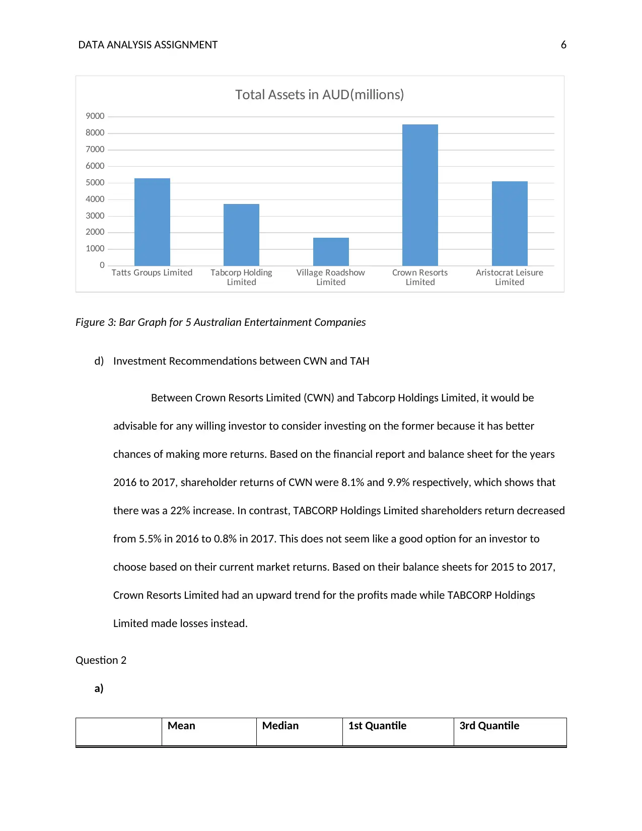
c) Bar graph for 5 entertainment companies in Australia

DATA ANALYSIS ASSIGNMENT 6
Tatts Groups Limited Tabcorp Holding
Limited Village Roadshow
Limited Crown Resorts
Limited Aristocrat Leisure
Limited
0
1000
2000
3000
4000
5000
6000
7000
8000
9000
Total Assets in AUD(millions)
Figure 3: Bar Graph for 5 Australian Entertainment Companies
d) Investment Recommendations between CWN and TAH
Between Crown Resorts Limited (CWN) and Tabcorp Holdings Limited, it would be
advisable for any willing investor to consider investing on the former because it has better
chances of making more returns. Based on the financial report and balance sheet for the years
2016 to 2017, shareholder returns of CWN were 8.1% and 9.9% respectively, which shows that
there was a 22% increase. In contrast, TABCORP Holdings Limited shareholders return decreased
from 5.5% in 2016 to 0.8% in 2017. This does not seem like a good option for an investor to
choose based on their current market returns. Based on their balance sheets for 2015 to 2017,
Crown Resorts Limited had an upward trend for the profits made while TABCORP Holdings
Limited made losses instead.
Question 2
a)
Mean Median 1st Quantile 3rd Quantile

DATA ANALYSIS ASSIGNMENT 7
CBA 3.1 3.05 2.49 3.7325
NAB 2.311167 2.359 2.1875 2.45075
ANZ 2.064818 2.048 1.91 2.173
WBC 2.0367 2.035 1.907 2.2355
b)
CBA NAB ANZ WBC
Standard Deviation 0.7540 0.2182 0.3421 0.3483
Range 2.23 0.785 1.206 1.304
Coefficient of Variation 24.32% 9.44% 16.57% 17.10%
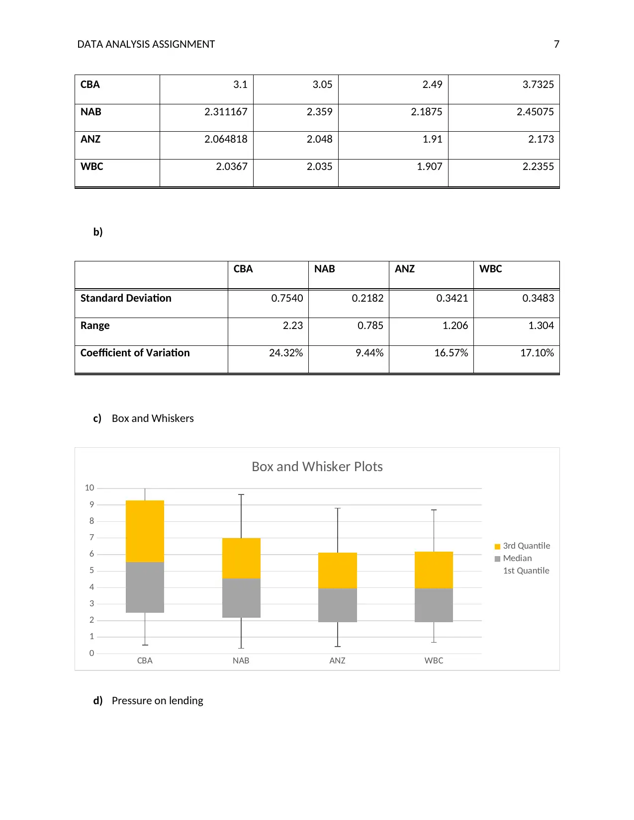
c) Box and Whiskers
CBA NAB ANZ WBC
0
1
2
3
4
5
6
7
8
9
10
Box and Whisker Plots
3rd Quantile
Median
1st Quantile
d) Pressure on lending

DATA ANALYSIS ASSIGNMENT 8
The pressure on lending generally affects the annual dividends differently on the banks.
For instance, CBA seems to be performing better than the other three based on the average
dividends per share and the range statistics. NAB, ANZ, and WBC are performing poorly as
compared to CBA. However, CBA has the highest variation of 24.32% in relation to 9.44%,
16.57% and 17.1% of NAB, ANZ, and WBC respectively. The lending pressure is aimed at
ensuring that the poorly performing banks can improve because of a base on CBA’s
performance, there is a good market for the banking sector.
Question 3
a) Society and culture are the most popular discipline for the best-performing students. With a
proportion of 8,180 /221,060 ¿ 3.7 %
b) The number students studying society and culture and are on ATAR score of less than 80 would
be2814+2807+3906+5030=14,557. Therefore, the probability of selecting a student with
ATAR score less than 80 who is studying society and culture would be 14,557
221,060 =0.0658 .
c) Society and culture discipline has the highest proportion of students with the lowest ATAR
grades. The proportion of students studying society and culture and having ATAR score of less
than 50 is 2,814
221,060 =0.0127.
d) Health discipline has the highest proportion of students with the highest proportion of students
in the category of No ATAR/Non-Yr 12.
 This is because students wishing to undertake any course in health discipline can be rated
based on their prerequisite studies.
 Also, those who are of No ATAR category can be accepted in the health discipline through
mature entry option and be engaged on special tertiary examinations.

DATA ANALYSIS ASSIGNMENT 9
Question 4
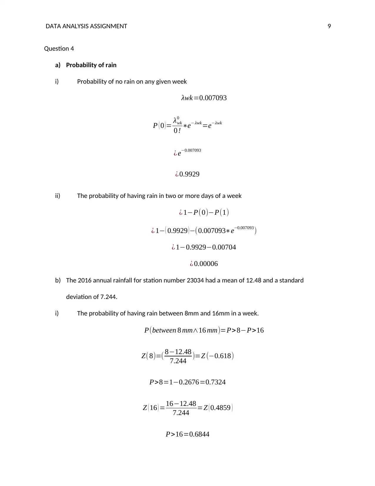
a) Probability of rain
i) Probability of no rain on any given week
λwk=0.007093
P ( 0 )= λwk
0
0 ! ∗e− λwk =e−λwk
¿ e−0.007093
¿ 0.9929
ii) The probability of having rain in two or more days of a week
¿ 1−P(0)−P(1)
¿ 1− ( 0.9929 )−(0.007093∗e−0.007093 )
¿ 1−0.9929−0.00704
¿ 0.00006
b) The 2016 annual rainfall for station number 23034 had a mean of 12.48 and a standard
deviation of 7.244.
i) The probability of having rain between 8mm and 16mm in a week.
P(between 8 mm∧16 mm)=P>8−P>16
Z( 8)=( 8−12.48
7.244 )=Z (−0.618)
P>8=1−0.2676=0.7324
Z ( 16 ) =16−12.48
7.244 =Z ( 0.4859 )
P>16=0.6844

DATA ANALYSIS ASSIGNMENT 10
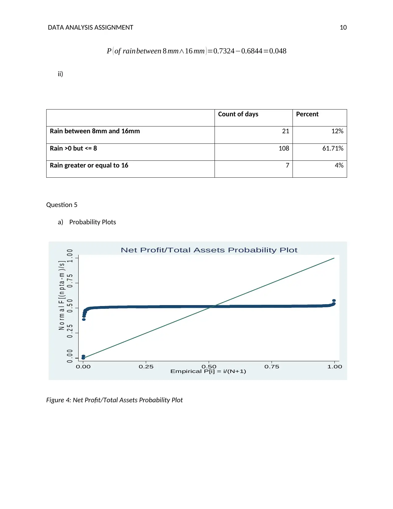
P ( of rainbetween 8 mm∧16 mm ) =0.7324−0.6844=0.048
ii)
Count of days Percent
Rain between 8mm and 16mm 21 12%
Rain >0 but <= 8 108 61.71%
Rain greater or equal to 16 7 4%
Question 5
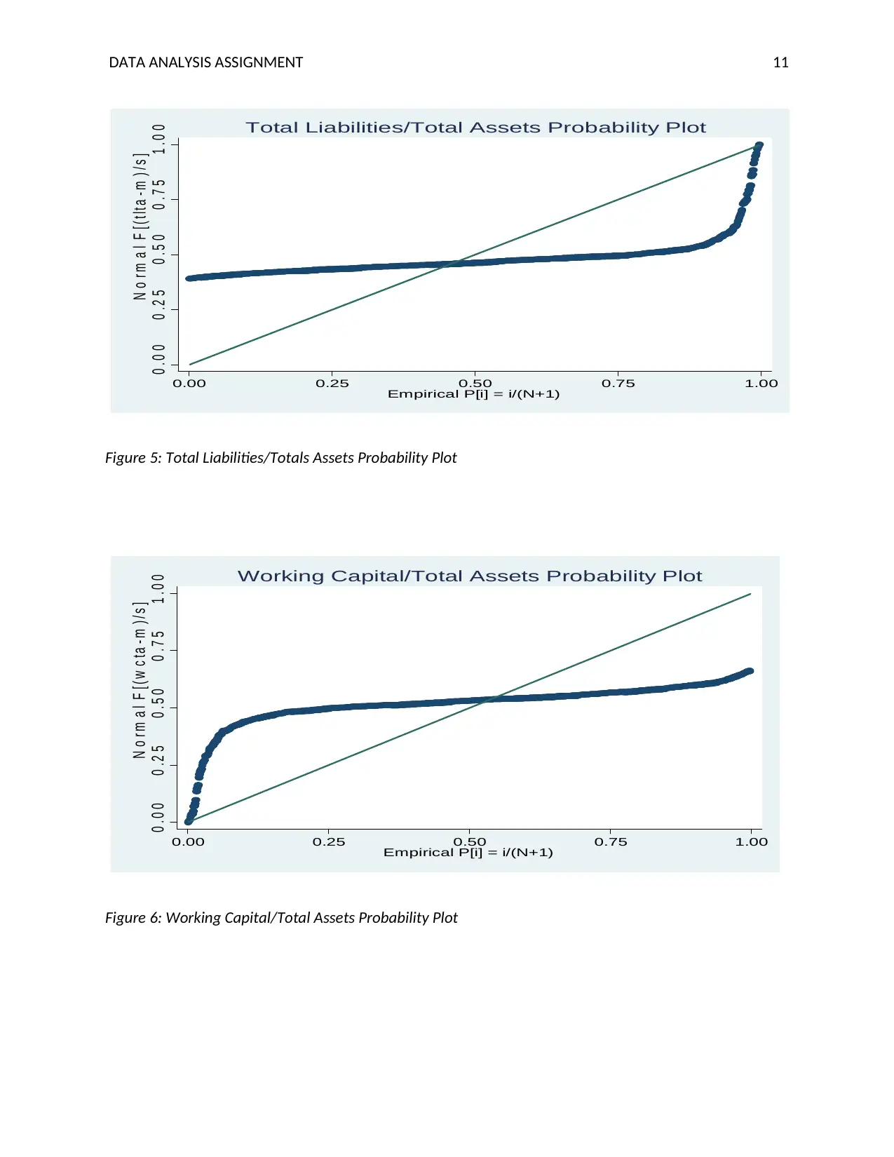
a) Probability Plots
0 . 0 0 0 . 2 5 0 . 5 0 0 . 7 5 1 . 0 0
N o r m a l F [ ( n p t a - m ) / s ]
0.00 0.25 0.50 0.75 1.00
Empirical P[i] = i/(N+1)
Net Profit/Total Assets Probability Plot
Figure 4: Net Profit/Total Assets Probability Plot

DATA ANALYSIS ASSIGNMENT 11
0 . 0 0 0 . 2 5 0 . 5 0 0 . 7 5 1 . 0 0
N o r m a l F [ ( t l t a - m ) / s ]
0.00 0.25 0.50 0.75 1.00
Empirical P[i] = i/(N+1)
Total Liabilities/Total Assets Probability Plot
Figure 5: Total Liabilities/Totals Assets Probability Plot
0 . 0 0 0 . 2 5 0 . 5 0 0 . 7 5 1 . 0 0
N o r m a l F [ ( w c t a - m ) / s ]
0.00 0.25 0.50 0.75 1.00
Empirical P[i] = i/(N+1)
Working Capital/Total Assets Probability Plot
Figure 6: Working Capital/Total Assets Probability Plot

DATA ANALYSIS ASSIGNMENT 12
0 . 0 0 0 . 2 5 0 . 5 0 0 . 7 5 1 . 0 0
N o r m a l F [ ( o e t l- m ) / s ]
0.00 0.25 0.50 0.75 1.00
Empirical P[i] = i/(N+1)
Operating Expenses/Total Liabilities Probability Plot
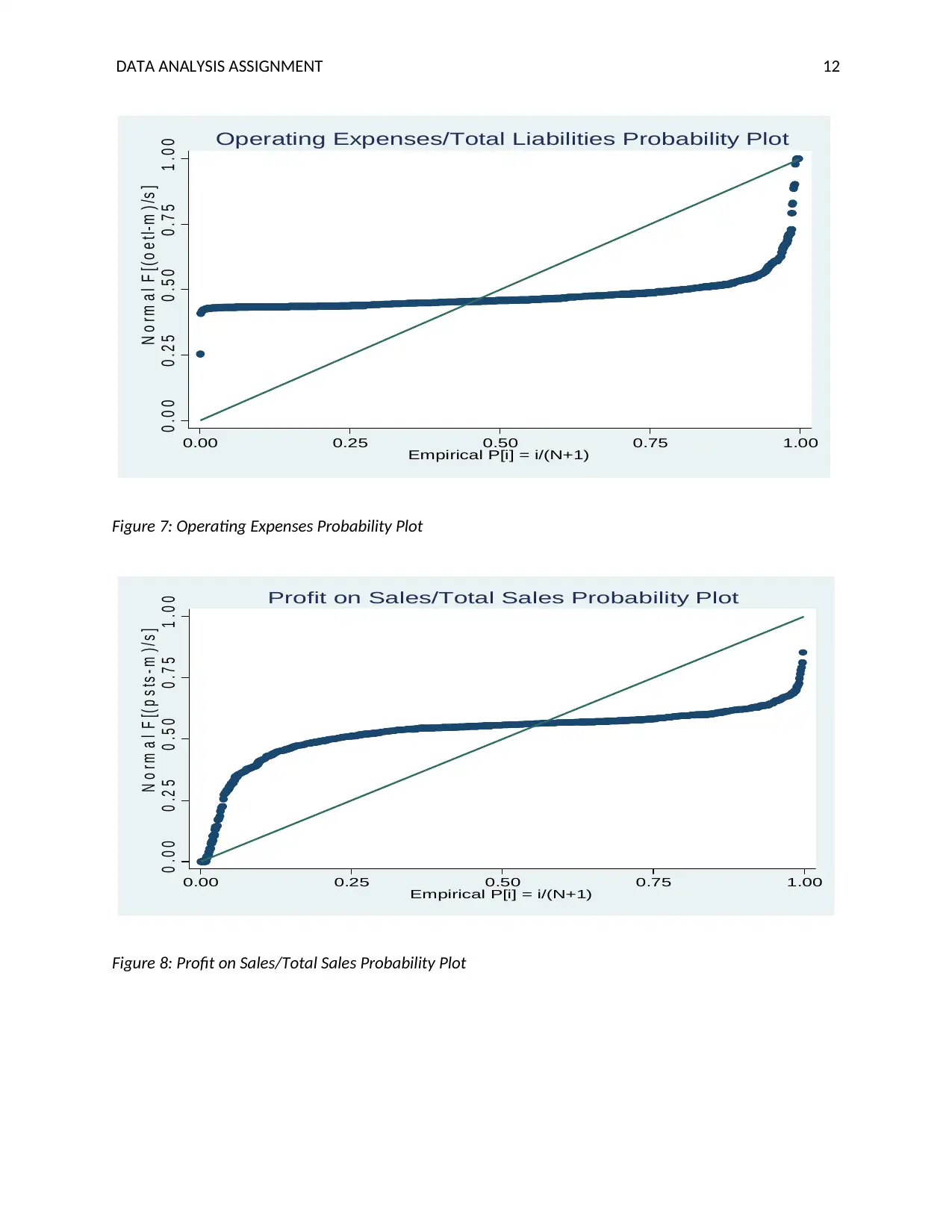
Figure 7: Operating Expenses Probability Plot
0 . 0 0 0 . 2 5 0 . 5 0 0 . 7 5 1 . 0 0
N o r m a l F [ ( p s t s - m ) / s ]
0.00 0.25 0.50 0.75 1.00
Empirical P[i] = i/(N+1)
Profit on Sales/Total Sales Probability Plot
Figure 8: Profit on Sales/Total Sales Probability Plot

DATA ANALYSIS ASSIGNMENT 13
0 . 0 0 0 . 2 5 0 . 5 0 0 . 7 5 1 . 0 0
N o r m a l F [ ( t c t s - m ) / s ]
0.00 0.25 0.50 0.75 1.00
Empirical P[i] = i/(N+1)
Total Costs/Total Sales Probability Plot
Figure 9: Total Costs/Total Sales Probability Plot
According to figures 4-9, the variables are not normally distributed because the dotted
points do not follow the diagonal line originating from the [0, 0] point in the Cartesian plane.
b) Confidence Intervals
Variable Observations Mean Std. Err. [95% Conf. Interval]
npta 909 -.57713 .5116146 -1.581215 .4269546
tlta 909 .808647 .0964677 .6193215 .9979725
wcta 909 -.0429552 .0829936 -.2058367 .1199263
oetl 909 5.312791 1.069064 3.214667 7.410915
psts 909 -.082214 .0241677 -.1296451 -.0347829
tcts 909 1.028756 .0277385 .9743171 1.083195
c) Hypothesis Testing
 Net Profit/Total Assets (NP/TA)

DATA ANALYSIS ASSIGNMENT 14
Group Observations Mean Std. Err. Std. Dev. [95% Conf. Interval]
0 501 .0698774 .0067548 .1511933 .0566061 .0831487
1 408 -1.371617 1.139354 23.01383 -3.611371 .868137
combined 909 -.57713 .5116146 15.42499 -1.581215 .4269546
diff 1.441494 1.139374 -.7982985 3.681287
diff = mean(0) - mean(1) t = 1.2652
Ho: diff = 0 Satterthwaite's degrees of freedom = 407.029
Ha: diff < 0 Ha: diff != 0 Ha: diff > 0
Pr(T < t) = 0.8967 Pr(|T| > |t|) = 0.2065 Pr(T > t) = 0.1033
The p-value for the two sided test is greater than 0.05, hence concluding that there is a
significant difference between those who were bankrupt and their counterparts based on their
net profit/Total assets ratio.
 Total Liabilities/Total Assets (TL/TA)
Group Observations Mean Std. Err. Std. Dev. [95% Conf. Interval]
0 501 .4743522 .0138999 .3111221 .4470427 .5016616
1 408 1.219141 .212632 4.294955 .8011474 1.637135
combined 909 .808647 .0964677 2.908464 .6193215 .9979725
diff -.7447892 .2130858 -1.163665 -.3259136
diff = mean(0) - mean(1) t = -3.4953
Ho: diff = 0 Satterthwaite's degrees of freedom = 410.48
Ha: diff < 0 Ha: diff != 0 Ha: diff > 0
Pr(T < t) = 0.0003 Pr(|T| > |t|) = 0.0005 Pr(T > t) = 0.9997

DATA ANALYSIS ASSIGNMENT 15
The p-value for the two-sample t-test is less than 0.05, hence concluding that there is a
significant difference between bankrupt and not bankrupt individuals based on the ratio of total
liabilities/total assets.
 Working Capital/Total Assets (WC/TA)
Group Observations Mean Std. Err. Std. Dev. [95% Conf. Interval]
0 501 .2358828 .0144696 .323873 .2074541 .2643114
1 408 -.3853519 .1827501 3.691372 -.7446039 -.0260999
combined 909 -.0429552 .0829936 2.502225 -.2058367 .1199263
diff .6212347 .1833221 .2608717 .9815976
diff = mean(0) - mean(1) t = 3.3888
Ho: diff = 0 Satterthwaite's degrees of freedom = 412.106
Ha: diff < 0 Ha: diff != 0 Ha: diff > 0
Pr(T < t) = 0.9996 Pr(|T| > |t|) = 0.0008 Pr(T > t) = 0.0004
The p-value is less than 0.05. There is a significant difference between bankrupt and
nonbankrupt based on the ratio of working capital and total assets.
 Operating Expenses/Total Liabilities (OE/TL)
Group Observations Mean Std. Err. Std. Dev. [95% Conf. Interval]
0 501 3.676291 .2622549 5.87006 3.161034 4.191549
1 408 7.322317 2.357744 47.62409 2.687441 11.95719
combined 909 5.312791 1.069064 32.23189 3.214667 7.410915

DATA ANALYSIS ASSIGNMENT 16
diff -3.646026 2.372285 -8.30915 1.017098
diff = mean(0) - mean(1) t = -1.5369
Ho: diff = 0 Satterthwaite's degrees of freedom = 417.081
Ha: diff < 0 Ha: diff != 0 Ha: diff > 0
Pr(T < t) = 0.0625 Pr(|T| > |t|) = 0.1251 Pr(T > t) = 0.9375
There is no difference between bankrupt and nonbankrupt based on ratio of operating
expenses and total liabilities
 Profit on Sales/Total Sales (PS/TS)
Group Observations Mean Std. Err. Std. Dev. [95% Conf. Interval]
0 501 .0535706 .0073132 .1636905 .0392023 .0679389
1 408 -.2489495 .0519473 1.049284 -.351068 -.146831
combined 909 -.082214 .0241677 .7286483 -.1296451 -.0347829
diff .3025201 .0524595 .1994063 .4056338
diff = mean(0) - mean(1) t = 5.7667
Ho: diff = 0 Satterthwaite's degrees of freedom = 423.157
Ha: diff < 0 Ha: diff != 0 Ha: diff > 0
Pr(T < t) = 1.0000 Pr(|T| > |t|) = 0.0000 Pr(T > t) = 0.0000
The test for the difference between bankrupt and nonbankrupt on the ratio of profit to
sales and total assets is very significant. This is because the p-value is less than 0.001 for the two
sided t-test.
 Total Costs/Total Sales (TC/TS)

DATA ANALYSIS ASSIGNMENT 17
Group Observations Mean Std. Err. Std. Dev. [95% Conf. Interval]
0 501 .9140897 .0071581 .1602206 .900026 .9281535
1 408 1.16956 .0604873 1.221784 1.050653 1.288466
combined 909 1.028756 .0277385 .8363067 .9743171 1.083195
diff -.2554701 .0609094 -.3751967 -.1357436
diff = mean(0) - mean(1) t = -4.1943
Ho: diff = 0 Satterthwaite's degrees of freedom = 418.413
Ha: diff < 0 Ha: diff != 0 Ha: diff > 0
Pr(T < t) = 0.0000 Pr(|T| > |t|) = 0.0000 Pr(T > t) = 1.0000
The p-value for the two-sided t-test is less than 0.05, hence concluding that there is a
significant difference between bankrupt and nonbankrupt on the basis of total costs/totals sales
ratio.