Econometric Methods FIN5EME: JNJ Stock Analysis - La Trobe University
VerifiedAdded on 2023/06/13
|11
|1053
|145
Homework Assignment
AI Summary
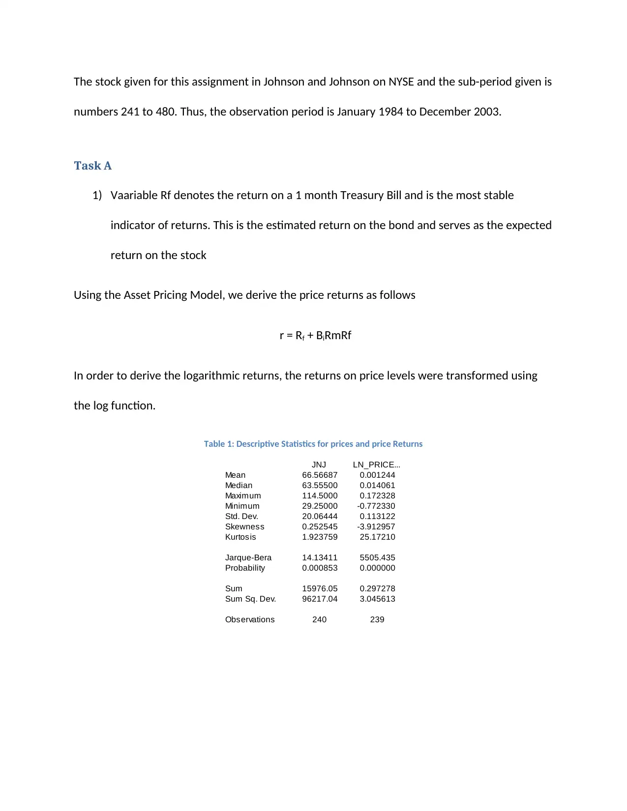
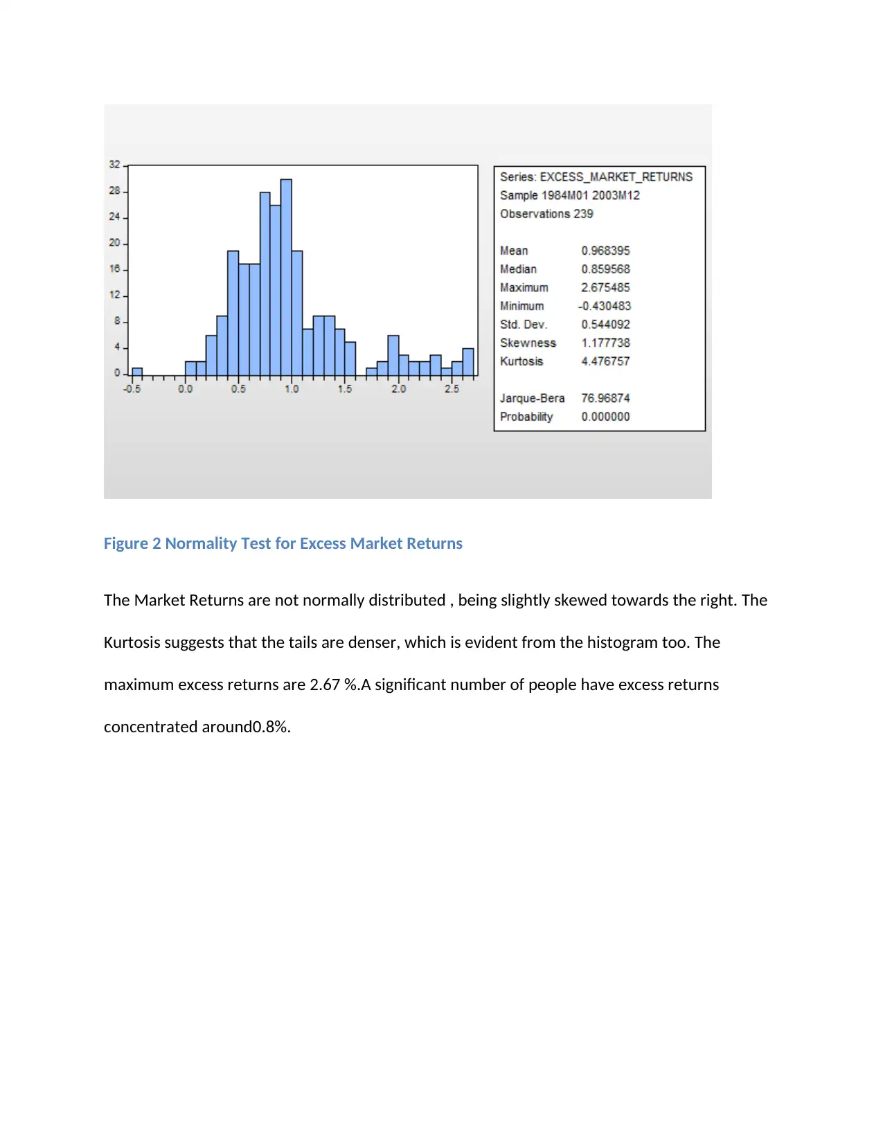
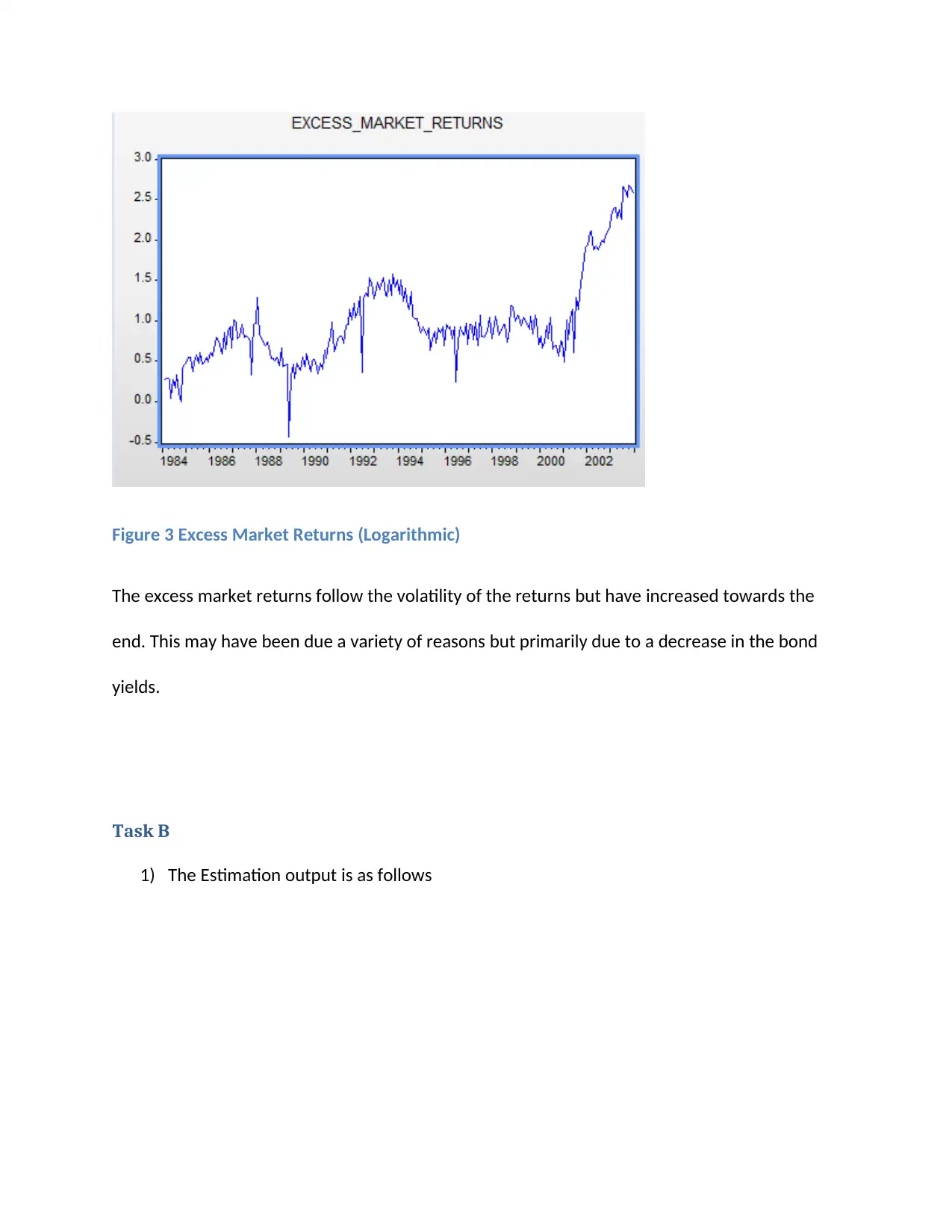
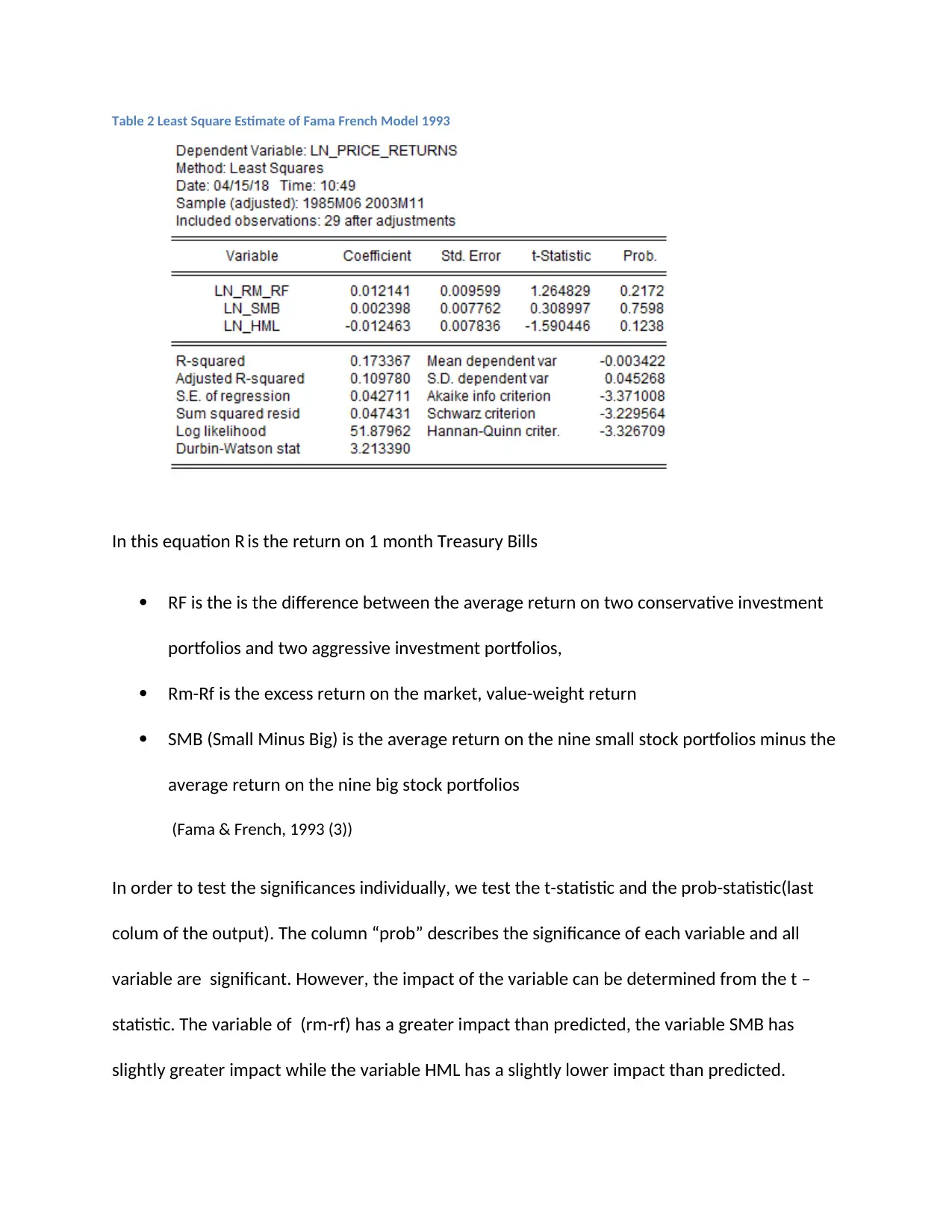
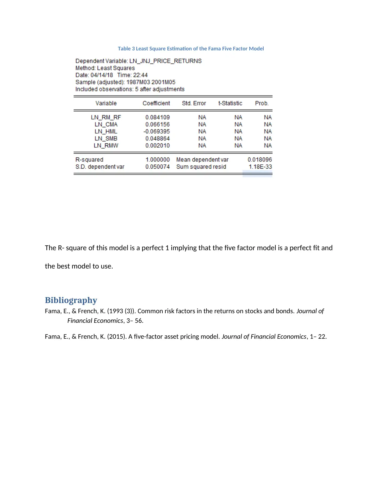
This assignment provides an econometric analysis of Johnson & Johnson (JNJ) stock using data from January 1984 to December 2003. Task A involves analyzing the descriptive statistics of price levels and logarithmic returns, time series plots, and normality tests for excess market returns. The analysis reveals non-normal distribution and volatility in price returns. Task B focuses on applying the Fama-French three-factor and five-factor models to estimate stock returns, evaluating the significance of variables, and interpreting the R-squared values. The five-factor model demonstrates a perfect fit. Desklib is a platform where you can find similar assignments and study resources.


1 out of 11
Your All-in-One AI-Powered Toolkit for Academic Success.
+13062052269
info@desklib.com
Available 24*7 on WhatsApp / Email
![[object Object]](/_next/static/media/star-bottom.7253800d.svg)
Copyright © 2020–2026 A2Z Services. All Rights Reserved. Developed and managed by ZUCOL.