Kinematic Modeling of a Tricycle Robot: Simulation and Analysis
VerifiedAdded on 2020/05/16
|26
|3301
|2504
Report
AI Summary
This report focuses on the kinematic modeling of a tricycle robot, exploring its movement based on control factors like speed and steering angle. It investigates two configurations: front wheel steering with rear wheel rolling, and front wheel steering and driving. The study utilizes MATLAB R2017a for simulations and includes MATLAB scripts for testing. The report details the building and simulation of the robot's kinematic model, along with localization using a particle filter. It discusses assumptions, results, and observations related to trajectory determination under varying parameters. The analysis covers the derivation of kinematic modeling equations, system model definition using experimental results, and the application of PID control strategies. The report also addresses trajectory control, steering control, and velocity control, including the design of a lead-lag compensator for achieving desired performance characteristics. The study compares the open loop performance of the robot with the model response, and analyzes the minimum turning radius. Finally, it describes the implementation of a discrete-time controller and the analysis of the closed loop performance.

university or college
Department or faculty
Date of submission
Students name student Id contribution to assignment
Department or faculty
Date of submission
Students name student Id contribution to assignment
Paraphrase This Document
Need a fresh take? Get an instant paraphrase of this document with our AI Paraphraser
EXECUTIVE SUMMARY
This paper seeks to perform kinematic modelling of a tricycle robot’s movement. Some of the
main control factors are the speed of motion of the tricycle as well as the steering angle. The
paper seeks to derive the kinematic modelling equations in two states where the front wheel does
the steering and the rear wheel roll over and where the front wheels do both the steering and
driving. The software used for this tests and simulations is the MATLAB R2017a. the MATLAB
scripts are appended alongside the report for testing purposes. The paper seeks to build and
simulate the kinematic model of the robot. It also seeks to determine the localization using a
particle filter. The discussion section highlights the main assumptions made in regards to this
report and it analyses the results and observations made in meeting the aims of the tests. The
paper seeks to determine the trajectory or the path the tricycle takes within a given period of time
when different parameters are altered to that effect. The derived system model has been
completely defined to use experimental results obtained for the robot tricycle design.
Page 1 of 26
TABLE OF CONTENTS
EXECUTIVE SUMMARY.........................................................................................................................1
BASIC OVERVIEW...................................................................................................................................3
RESULTS & OBSERVATIONS.................................................................................................................6
DISCUSSION...........................................................................................................................................21
CONCLUSION.........................................................................................................................................24
RECOMMENDATIONS AND FUTURE WORK....................................................................................24
REFERENCES..........................................................................................................................................25
Page 2 of 26
⊘ This is a preview!⊘
Do you want full access?
Subscribe today to unlock all pages.
Trusted by 1+ million students worldwide
BASIC OVERVIEW
There has been a great development in the artificial intelligence and robotics field. The focus
now is on enabling better control strategies to achieve robust and optimal performance. The three
wheeled vehicles are mainly used in the local public transport globally but they tend to lag
behind in terms of speed and steering angles although they have merits in localization and
navigation. In most systems in the industry, the PID is used to ensure control of the system.
Some other applications are such as the self-driving car which was designed by google and has
now been built by other car companies globally (Folsom, 2013). The car is already commuting in
various states and roads nationwide and they are strict in the aerodynamic design features as
those could affect the motion. The aerodynamic considerations are basically involved in the
dynamic modelling of a system as opposed to the kinematic modelling as is the focus in this
report (Mercedes-Benz, 2016). For instance, currently the Mercedes Benz company is working
on an electric vehicle in relation with a mechanical design. One of the key challenges faced by
many vehicle companies is in the monitoring of the control and stability of a vehicle after design.
The dynamic modelling seeks to discuss the stability factor of the three-wheeled vehicle as
designed but the control and speed variations are focused on in the kinematic modelling. It is
crucial to note that the highest number of robot locomotives are based on the differential drive
model. The model states that the two powered wheels are used to drive the robot as well as
change its direction, hence they are used for both driving and steering. The control strategies for
the differential drive model of the robot are completely different and do not apply to other robot
designs such as the Ackerman drive robots or the omnidirectional mobile robots. Another model
of locomotion for the three-wheeled robot tricycle is where the steering and powering is done at
the front wheels (Miyazaki, et al., n.d.). The advantage of the steering geometry has several
advantages for the purpose of localization and motion planning.
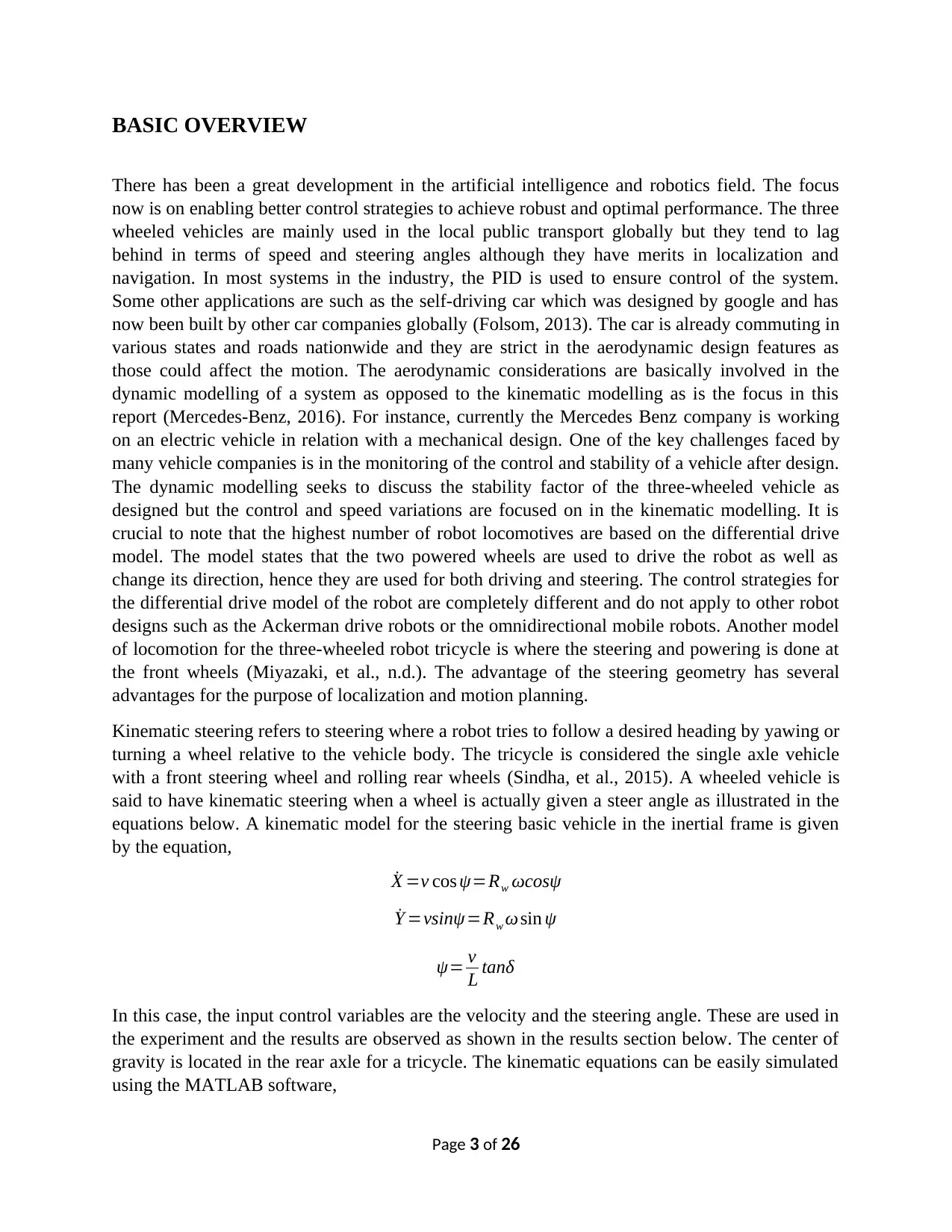
Kinematic steering refers to steering where a robot tries to follow a desired heading by yawing or
turning a wheel relative to the vehicle body. The tricycle is considered the single axle vehicle
with a front steering wheel and rolling rear wheels (Sindha, et al., 2015). A wheeled vehicle is
said to have kinematic steering when a wheel is actually given a steer angle as illustrated in the
equations below. A kinematic model for the steering basic vehicle in the inertial frame is given
by the equation,
˙X =v cos ψ=Rw ωcosψ
˙Y =vsinψ=Rw ω sin ψ
ψ= v
L tanδ
In this case, the input control variables are the velocity and the steering angle. These are used in
the experiment and the results are observed as shown in the results section below. The center of
gravity is located in the rear axle for a tricycle. The kinematic equations can be easily simulated
using the MATLAB software,
Page 3 of 26
There has been a great development in the artificial intelligence and robotics field. The focus
now is on enabling better control strategies to achieve robust and optimal performance. The three
wheeled vehicles are mainly used in the local public transport globally but they tend to lag
behind in terms of speed and steering angles although they have merits in localization and
navigation. In most systems in the industry, the PID is used to ensure control of the system.
Some other applications are such as the self-driving car which was designed by google and has
now been built by other car companies globally (Folsom, 2013). The car is already commuting in
various states and roads nationwide and they are strict in the aerodynamic design features as
those could affect the motion. The aerodynamic considerations are basically involved in the
dynamic modelling of a system as opposed to the kinematic modelling as is the focus in this
report (Mercedes-Benz, 2016). For instance, currently the Mercedes Benz company is working
on an electric vehicle in relation with a mechanical design. One of the key challenges faced by
many vehicle companies is in the monitoring of the control and stability of a vehicle after design.
The dynamic modelling seeks to discuss the stability factor of the three-wheeled vehicle as
designed but the control and speed variations are focused on in the kinematic modelling. It is
crucial to note that the highest number of robot locomotives are based on the differential drive
model. The model states that the two powered wheels are used to drive the robot as well as
change its direction, hence they are used for both driving and steering. The control strategies for
the differential drive model of the robot are completely different and do not apply to other robot
designs such as the Ackerman drive robots or the omnidirectional mobile robots. Another model
of locomotion for the three-wheeled robot tricycle is where the steering and powering is done at
the front wheels (Miyazaki, et al., n.d.). The advantage of the steering geometry has several
advantages for the purpose of localization and motion planning.
Kinematic steering refers to steering where a robot tries to follow a desired heading by yawing or
turning a wheel relative to the vehicle body. The tricycle is considered the single axle vehicle
with a front steering wheel and rolling rear wheels (Sindha, et al., 2015). A wheeled vehicle is
said to have kinematic steering when a wheel is actually given a steer angle as illustrated in the
equations below. A kinematic model for the steering basic vehicle in the inertial frame is given
by the equation,
˙X =v cos ψ=Rw ωcosψ
˙Y =vsinψ=Rw ω sin ψ
ψ= v
L tanδ
In this case, the input control variables are the velocity and the steering angle. These are used in
the experiment and the results are observed as shown in the results section below. The center of
gravity is located in the rear axle for a tricycle. The kinematic equations can be easily simulated
using the MATLAB software,
Page 3 of 26
Paraphrase This Document
Need a fresh take? Get an instant paraphrase of this document with our AI Paraphraser
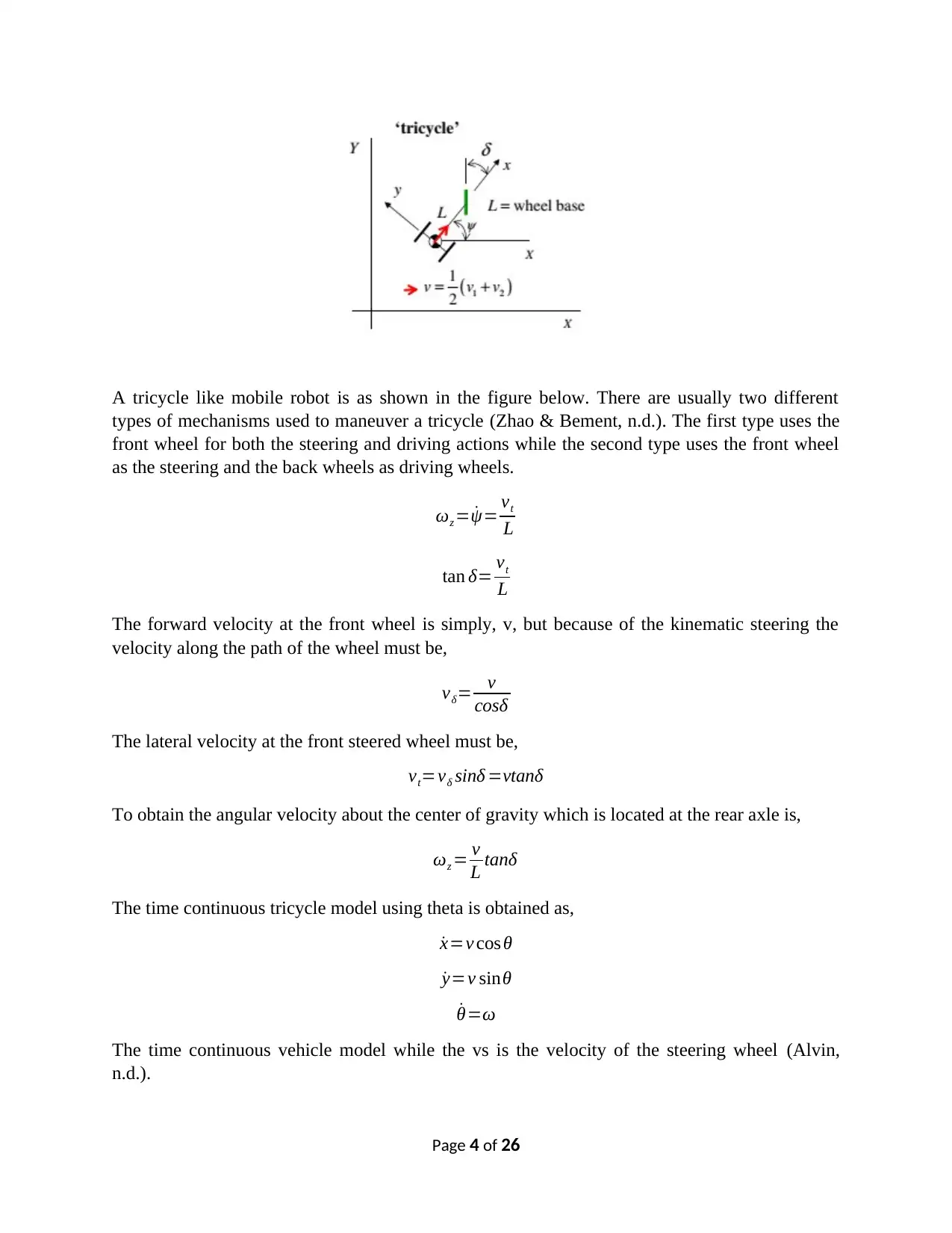
A tricycle like mobile robot is as shown in the figure below. There are usually two different
types of mechanisms used to maneuver a tricycle (Zhao & Bement, n.d.). The first type uses the
front wheel for both the steering and driving actions while the second type uses the front wheel
as the steering and the back wheels as driving wheels.
ωz = ˙ψ= vt
L
tan δ= vt
L
The forward velocity at the front wheel is simply, v, but because of the kinematic steering the
velocity along the path of the wheel must be,
vδ= v
cosδ
The lateral velocity at the front steered wheel must be,
vt=vδ sinδ =vtanδ
To obtain the angular velocity about the center of gravity which is located at the rear axle is,
ωz = v
L tanδ
The time continuous tricycle model using theta is obtained as,
˙x=v cosθ
˙y=v sinθ
˙θ=ω
The time continuous vehicle model while the vs is the velocity of the steering wheel (Alvin,
n.d.).
Page 4 of 26
In as much as we are keen on defining the trajectory of the locomotive, there is need to
determine the center of curvature on the path the robot traverse. The curvature of the path is the
inverse of the instantaneous radius of curvature. It is centered about the supposed center of a
circle. It is known as the ICC and is the center of a circle which passes through the path a given
point which has the same tangent and curvature at that point on the path. The absence of
actuators in the wheels gives way to precise localization which in turn helps in better trajectory
following and navigation of the vehicle. The modified mechanical design has its merits in the
navigation, in as much as it poses huge drawbacks in the modeling and control strategies
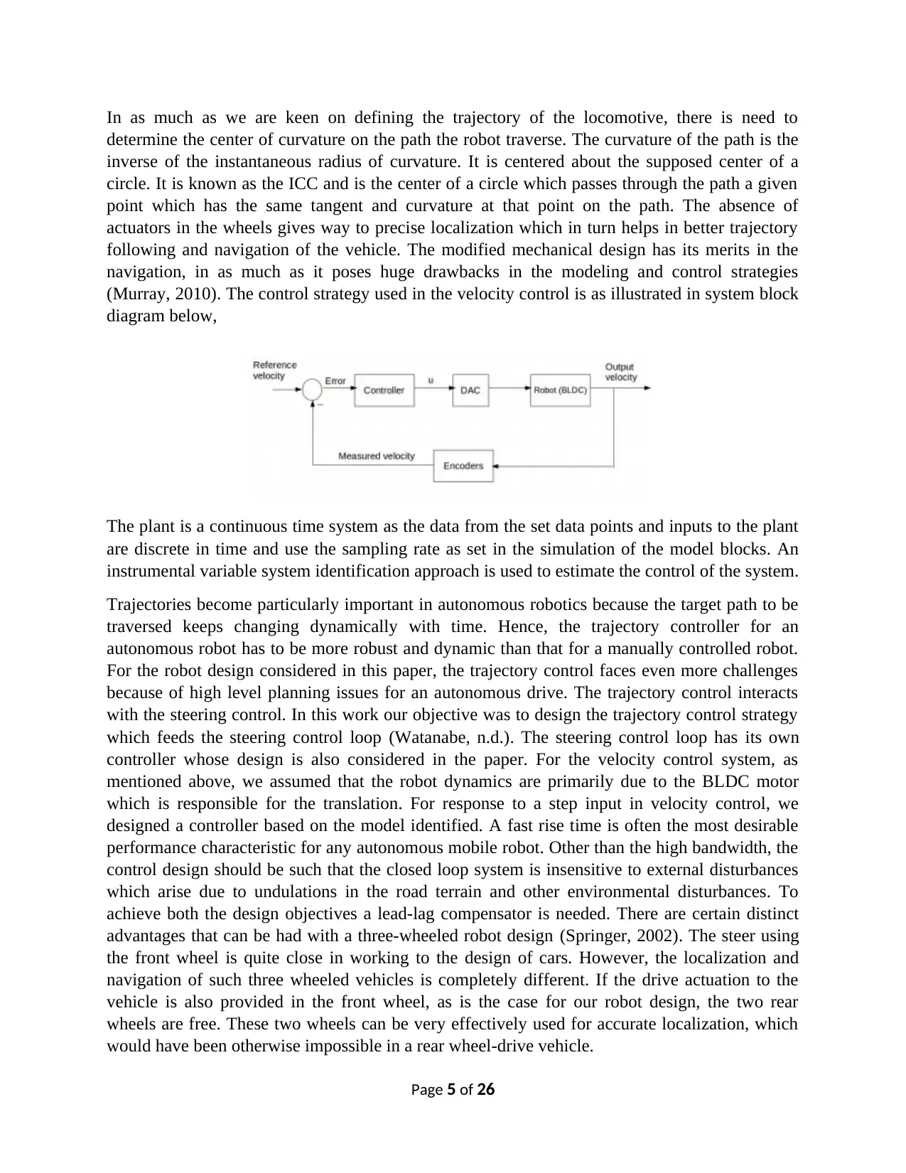
(Murray, 2010). The control strategy used in the velocity control is as illustrated in system block
diagram below,
The plant is a continuous time system as the data from the set data points and inputs to the plant
are discrete in time and use the sampling rate as set in the simulation of the model blocks. An
instrumental variable system identification approach is used to estimate the control of the system.
Trajectories become particularly important in autonomous robotics because the target path to be
traversed keeps changing dynamically with time. Hence, the trajectory controller for an
autonomous robot has to be more robust and dynamic than that for a manually controlled robot.
For the robot design considered in this paper, the trajectory control faces even more challenges
because of high level planning issues for an autonomous drive. The trajectory control interacts
with the steering control. In this work our objective was to design the trajectory control strategy
which feeds the steering control loop (Watanabe, n.d.). The steering control loop has its own
controller whose design is also considered in the paper. For the velocity control system, as
mentioned above, we assumed that the robot dynamics are primarily due to the BLDC motor
which is responsible for the translation. For response to a step input in velocity control, we
designed a controller based on the model identified. A fast rise time is often the most desirable
performance characteristic for any autonomous mobile robot. Other than the high bandwidth, the
control design should be such that the closed loop system is insensitive to external disturbances
which arise due to undulations in the road terrain and other environmental disturbances. To
achieve both the design objectives a lead-lag compensator is needed. There are certain distinct
advantages that can be had with a three-wheeled robot design (Springer, 2002). The steer using
the front wheel is quite close in working to the design of cars. However, the localization and
navigation of such three wheeled vehicles is completely different. If the drive actuation to the
vehicle is also provided in the front wheel, as is the case for our robot design, the two rear
wheels are free. These two wheels can be very effectively used for accurate localization, which
would have been otherwise impossible in a rear wheel-drive vehicle.
Page 5 of 26
determine the center of curvature on the path the robot traverse. The curvature of the path is the
inverse of the instantaneous radius of curvature. It is centered about the supposed center of a
circle. It is known as the ICC and is the center of a circle which passes through the path a given
point which has the same tangent and curvature at that point on the path. The absence of
actuators in the wheels gives way to precise localization which in turn helps in better trajectory
following and navigation of the vehicle. The modified mechanical design has its merits in the
navigation, in as much as it poses huge drawbacks in the modeling and control strategies
(Murray, 2010). The control strategy used in the velocity control is as illustrated in system block
diagram below,
The plant is a continuous time system as the data from the set data points and inputs to the plant
are discrete in time and use the sampling rate as set in the simulation of the model blocks. An
instrumental variable system identification approach is used to estimate the control of the system.
Trajectories become particularly important in autonomous robotics because the target path to be
traversed keeps changing dynamically with time. Hence, the trajectory controller for an
autonomous robot has to be more robust and dynamic than that for a manually controlled robot.
For the robot design considered in this paper, the trajectory control faces even more challenges
because of high level planning issues for an autonomous drive. The trajectory control interacts
with the steering control. In this work our objective was to design the trajectory control strategy
which feeds the steering control loop (Watanabe, n.d.). The steering control loop has its own
controller whose design is also considered in the paper. For the velocity control system, as
mentioned above, we assumed that the robot dynamics are primarily due to the BLDC motor
which is responsible for the translation. For response to a step input in velocity control, we
designed a controller based on the model identified. A fast rise time is often the most desirable
performance characteristic for any autonomous mobile robot. Other than the high bandwidth, the
control design should be such that the closed loop system is insensitive to external disturbances
which arise due to undulations in the road terrain and other environmental disturbances. To
achieve both the design objectives a lead-lag compensator is needed. There are certain distinct
advantages that can be had with a three-wheeled robot design (Springer, 2002). The steer using
the front wheel is quite close in working to the design of cars. However, the localization and
navigation of such three wheeled vehicles is completely different. If the drive actuation to the
vehicle is also provided in the front wheel, as is the case for our robot design, the two rear
wheels are free. These two wheels can be very effectively used for accurate localization, which
would have been otherwise impossible in a rear wheel-drive vehicle.
Page 5 of 26
⊘ This is a preview!⊘
Do you want full access?
Subscribe today to unlock all pages.
Trusted by 1+ million students worldwide
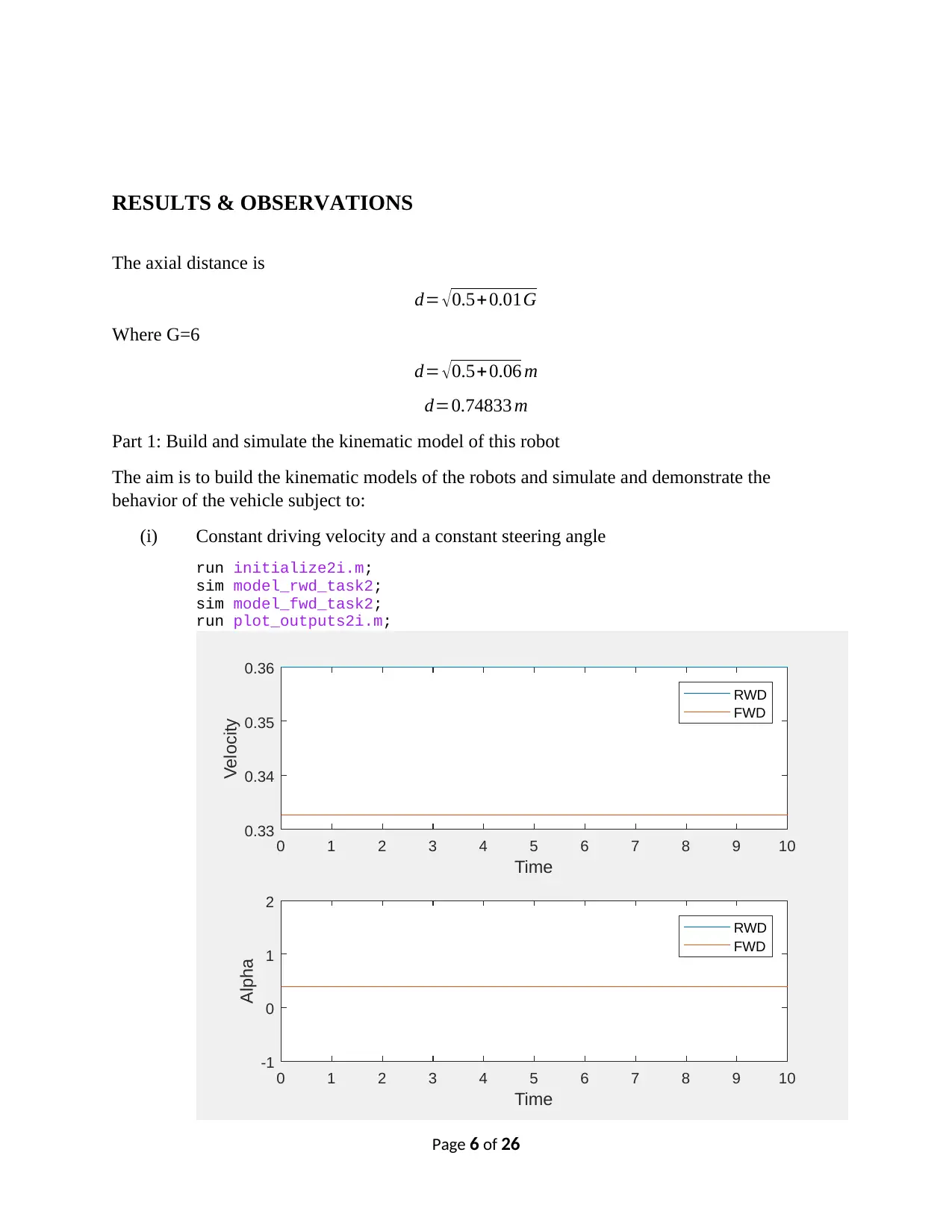
RESULTS & OBSERVATIONS
The axial distance is
d= √ 0.5+ 0.01G
Where G=6
d= √0.5+0.06 m
d=0.74833 m
Part 1: Build and simulate the kinematic model of this robot
The aim is to build the kinematic models of the robots and simulate and demonstrate the
behavior of the vehicle subject to:
(i) Constant driving velocity and a constant steering angle
run initialize2i.m;
sim model_rwd_task2;
sim model_fwd_task2;
run plot_outputs2i.m;
0 1 2 3 4 5 6 7 8 9 10
Time
0.33
0.34
0.35
0.36
Velocity
RWD
FWD
0 1 2 3 4 5 6 7 8 9 10
Time
-1
0
1
2
Alpha
RWD
FWD
Page 6 of 26
Paraphrase This Document
Need a fresh take? Get an instant paraphrase of this document with our AI Paraphraser
0 1 2 3 4 5 6 7 8 9 10
Time
0
1
2
Theta RWD
FWD
0 1 2 3 4 5 6 7 8 9 10
Time
0
2
4
Position Y
RWD
FWD
0 1 2 3 4 5 6 7 8 9 10
Time
0
1
2
Position X
RWD
FWD
0 0.2 0.4 0.6 0.8 1 1.2 1.4 1.6 1.8 2
X
0
0.5
1
1.5
2
2.5
3
Y
RWD
FWD
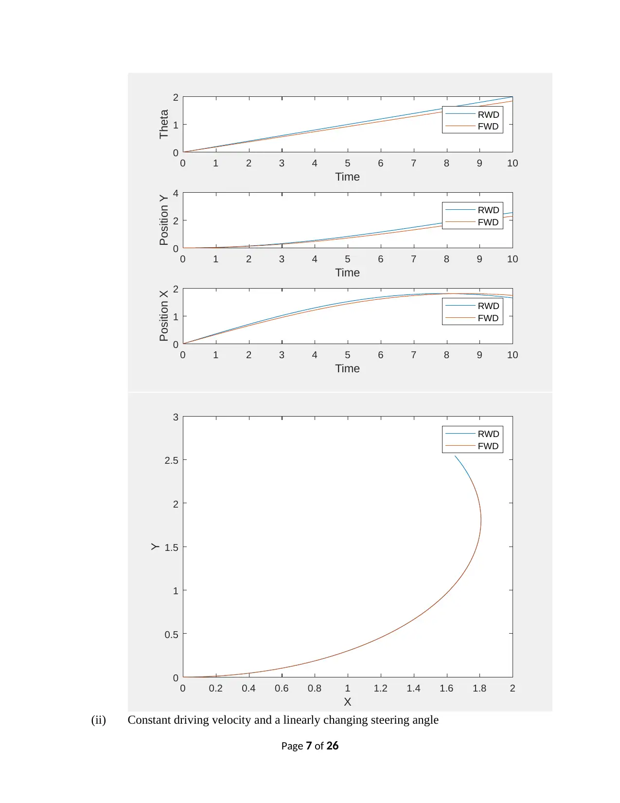
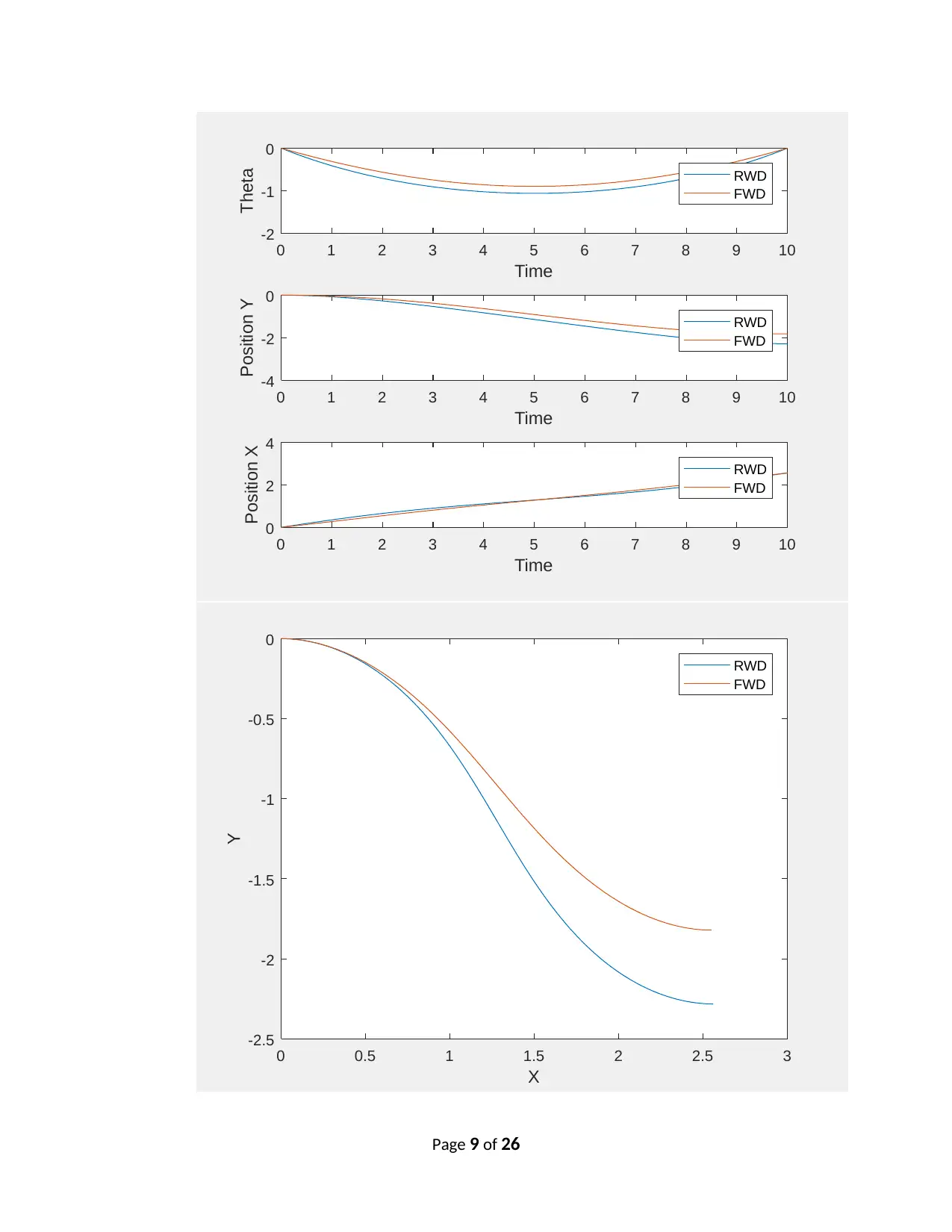
(ii) Constant driving velocity and a linearly changing steering angle
Page 7 of 26
Time
0
1
2
Theta RWD
FWD
0 1 2 3 4 5 6 7 8 9 10
Time
0
2
4
Position Y
RWD
FWD
0 1 2 3 4 5 6 7 8 9 10
Time
0
1
2
Position X
RWD
FWD
0 0.2 0.4 0.6 0.8 1 1.2 1.4 1.6 1.8 2
X
0
0.5
1
1.5
2
2.5
3
Y
RWD
FWD
(ii) Constant driving velocity and a linearly changing steering angle
Page 7 of 26
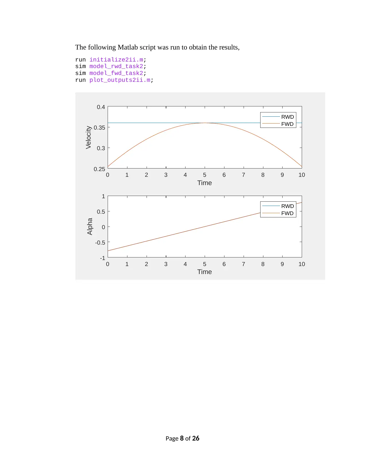
The following Matlab script was run to obtain the results,
run initialize2ii.m;
sim model_rwd_task2;
sim model_fwd_task2;
run plot_outputs2ii.m;
0 1 2 3 4 5 6 7 8 9 10
Time
0.25
0.3
0.35
0.4
Velocity
RWD
FWD
0 1 2 3 4 5 6 7 8 9 10
Time
-1
-0.5
0
0.5
1
Alpha
RWD
FWD
Page 8 of 26
run initialize2ii.m;
sim model_rwd_task2;
sim model_fwd_task2;
run plot_outputs2ii.m;
0 1 2 3 4 5 6 7 8 9 10
Time
0.25
0.3
0.35
0.4
Velocity
RWD
FWD
0 1 2 3 4 5 6 7 8 9 10
Time
-1
-0.5
0
0.5
1
Alpha
RWD
FWD
Page 8 of 26
⊘ This is a preview!⊘
Do you want full access?
Subscribe today to unlock all pages.
Trusted by 1+ million students worldwide
0 1 2 3 4 5 6 7 8 9 10
Time
-2
-1
0
Theta RWD
FWD
0 1 2 3 4 5 6 7 8 9 10
Time
-4
-2
0
Position Y
RWD
FWD
0 1 2 3 4 5 6 7 8 9 10
Time
0
2
4
Position X
RWD
FWD
0 0.5 1 1.5 2 2.5 3
X
-2.5
-2
-1.5
-1
-0.5
0
Y
RWD
FWD
Page 9 of 26
Time
-2
-1
0
Theta RWD
FWD
0 1 2 3 4 5 6 7 8 9 10
Time
-4
-2
0
Position Y
RWD
FWD
0 1 2 3 4 5 6 7 8 9 10
Time
0
2
4
Position X
RWD
FWD
0 0.5 1 1.5 2 2.5 3
X
-2.5
-2
-1.5
-1
-0.5
0
Y
RWD
FWD
Page 9 of 26
Paraphrase This Document
Need a fresh take? Get an instant paraphrase of this document with our AI Paraphraser
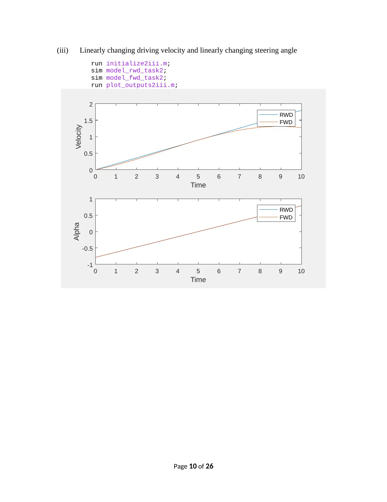
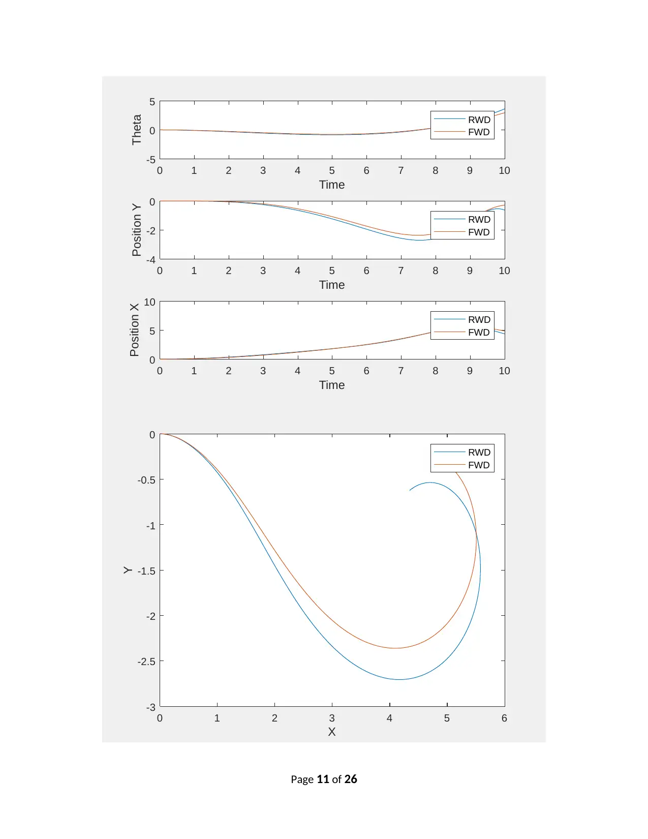
(iii) Linearly changing driving velocity and linearly changing steering angle
run initialize2iii.m;
sim model_rwd_task2;
sim model_fwd_task2;
run plot_outputs2iii.m;
0 1 2 3 4 5 6 7 8 9 10
Time
0
0.5
1
1.5
2
Velocity
RWD
FWD
0 1 2 3 4 5 6 7 8 9 10
Time
-1
-0.5
0
0.5
1
Alpha
RWD
FWD
Page 10 of 26
run initialize2iii.m;
sim model_rwd_task2;
sim model_fwd_task2;
run plot_outputs2iii.m;
0 1 2 3 4 5 6 7 8 9 10
Time
0
0.5
1
1.5
2
Velocity
RWD
FWD
0 1 2 3 4 5 6 7 8 9 10
Time
-1
-0.5
0
0.5
1
Alpha
RWD
FWD
Page 10 of 26
0 1 2 3 4 5 6 7 8 9 10
Time
-5
0
5
Theta RWD
FWD
0 1 2 3 4 5 6 7 8 9 10
Time
-4
-2
0
Position Y
RWD
FWD
0 1 2 3 4 5 6 7 8 9 10
Time
0
5
10
Position X
RWD
FWD
0 1 2 3 4 5 6
X
-3
-2.5
-2
-1.5
-1
-0.5
0
Y
RWD
FWD
Page 11 of 26
Time
-5
0
5
Theta RWD
FWD
0 1 2 3 4 5 6 7 8 9 10
Time
-4
-2
0
Position Y
RWD
FWD
0 1 2 3 4 5 6 7 8 9 10
Time
0
5
10
Position X
RWD
FWD
0 1 2 3 4 5 6
X
-3
-2.5
-2
-1.5
-1
-0.5
0
Y
RWD
FWD
Page 11 of 26
⊘ This is a preview!⊘
Do you want full access?
Subscribe today to unlock all pages.
Trusted by 1+ million students worldwide
1 out of 26