Regression Analysis: TA, ABC Total, Gender and Statistical Anxiety

This report presents regression analysis between TA, ABC Total, Gender and Statistical anxiety to determine the predictive relationship. The report includes the regression statistics, interpretation of the results, and the significance of the findings. The regression analysis helps in understanding the relationship between the variables and their impact on statistical anxiety.

Lab report
(Regression)

Contents
INTRODUCTION...........................................................................................................................3
MAIN BODY...................................................................................................................................3
Regression analysis between TA and Statistical anxiety.......................................................3
Regression analysis between ABC Total and Statistical anxiety...........................................4
Regression analysis between Gender and Statistical anxiety.................................................6
CONCLUSION................................................................................................................................9
REFERENCES..............................................................................................................................10

INTRODUCTION
In stats, the linear regression model is being used to discover patterns and trends in a particular
collected data. It may assume that there have been a relation among how much a user work and
how much they receive salary; regression test can support to measure that relation. Regression
analysis can also provide specific graph valid equation, which is further beneficial to forecast the
results (Morris, 2015).
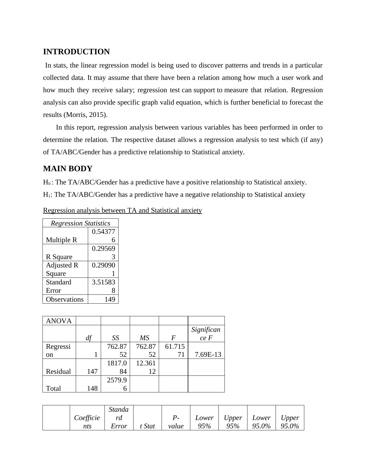
In this report, regression analysis between various variables has been performed in order to
determine the relation. The respective dataset allows a regression analysis to test which (if any)
of TA/ABC/Gender has a predictive relationship to Statistical anxiety.
MAIN BODY
H0 : The TA/ABC/Gender has a predictive have a positive relationship to Statistical anxiety.
H1: The TA/ABC/Gender has a predictive have a negative relationship to Statistical anxiety
Regression analysis between TA and Statistical anxiety
Regression Statistics
Multiple R
0.54377
6
R Square
0.29569
3
Adjusted R
Square
0.29090
1
Standard
Error
3.51583
8
Observations 149
ANOVA
df SS MS F
Significan
ce F
Regressi
on 1
762.87
52
762.87
52
61.715
71 7.69E-13
Residual 147
1817.0
84
12.361
12
Total 148
2579.9
6
Coefficie
nts
Standa
rd
Error t Stat
P-
value
Lower
95%
Upper
95%
Lower
95.0%
Upper
95.0%

Interce
pt 4.579819
1.2083
18
3.7902
43
0.0002
19 2.1919
6.9677
37 2.1919
6.9677
37
32 0.324423
0.0412
97
7.8559
35
7.69E-
13
0.2428
11
0.4060
35
0.2428
11
0.4060
35
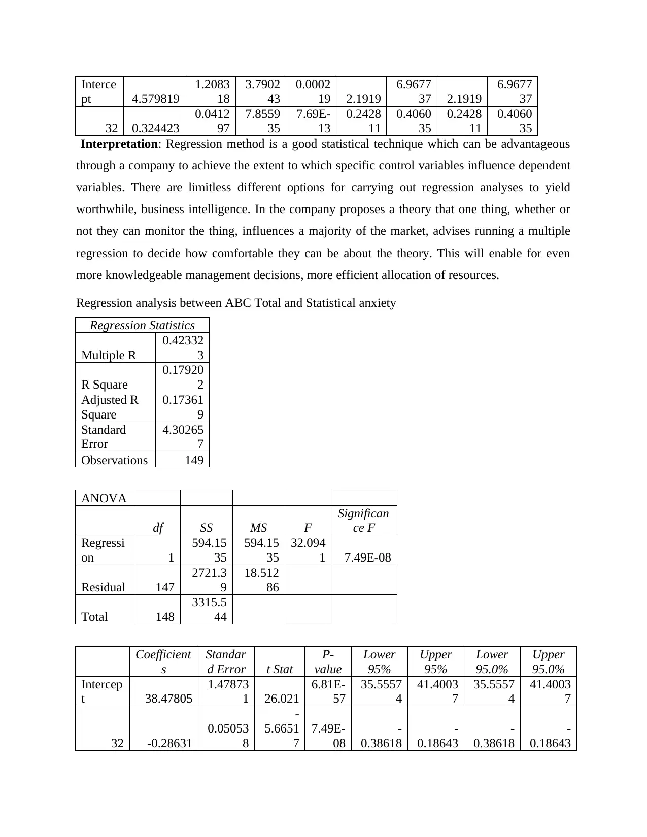
Interpretation: Regression method is a good statistical technique which can be advantageous
through a company to achieve the extent to which specific control variables influence dependent
variables. There are limitless different options for carrying out regression analyses to yield
worthwhile, business intelligence. In the company proposes a theory that one thing, whether or
not they can monitor the thing, influences a majority of the market, advises running a multiple
regression to decide how comfortable they can be about the theory. This will enable for even
more knowledgeable management decisions, more efficient allocation of resources.
Regression analysis between ABC Total and Statistical anxiety
Regression Statistics
Multiple R
0.42332
3
R Square
0.17920
2
Adjusted R
Square
0.17361
9
Standard
Error
4.30265
7
Observations 149
ANOVA
df SS MS F
Significan
ce F
Regressi
on 1
594.15
35
594.15
35
32.094
1 7.49E-08
Residual 147
2721.3
9
18.512
86
Total 148
3315.5
44
Coefficient
s
Standar
d Error t Stat
P-
value
Lower
95%
Upper
95%
Lower
95.0%
Upper
95.0%
Intercep
t 38.47805
1.47873
1 26.021
6.81E-
57
35.5557
4
41.4003
7
35.5557
4
41.4003
7
32 -0.28631
0.05053
8
-
5.6651
7
7.49E-
08
-
0.38618
-
0.18643
-
0.38618
-
0.18643

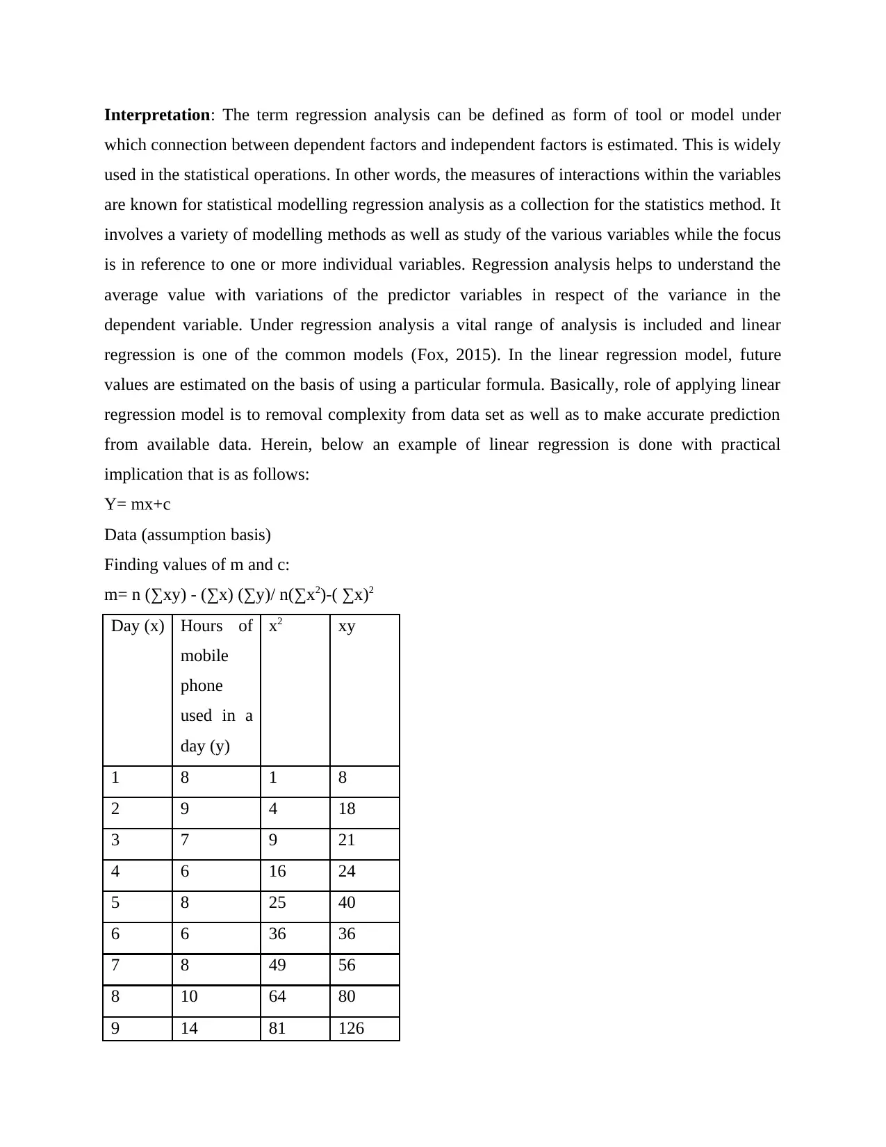
Interpretation: The term regression analysis can be defined as form of tool or model under
which connection between dependent factors and independent factors is estimated. This is widely
used in the statistical operations. In other words, the measures of interactions within the variables
are known for statistical modelling regression analysis as a collection for the statistics method. It
involves a variety of modelling methods as well as study of the various variables while the focus
is in reference to one or more individual variables. Regression analysis helps to understand the
average value with variations of the predictor variables in respect of the variance in the
dependent variable. Under regression analysis a vital range of analysis is included and linear
regression is one of the common models (Fox, 2015). In the linear regression model, future
values are estimated on the basis of using a particular formula. Basically, role of applying linear
regression model is to removal complexity from data set as well as to make accurate prediction
from available data. Herein, below an example of linear regression is done with practical
implication that is as follows:
Y= mx+c
Data (assumption basis)
Finding values of m and c:
m= n (∑xy) - (∑x) (∑y)/ n(∑x2)-( ∑x)2
Day (x) Hours of
mobile
phone
used in a
day (y)
x2 xy
1 8 1 8
2 9 4 18
3 7 9 21
4 6 16 24
5 8 25 40
6 6 36 36
7 8 49 56
8 10 64 80
9 14 81 126

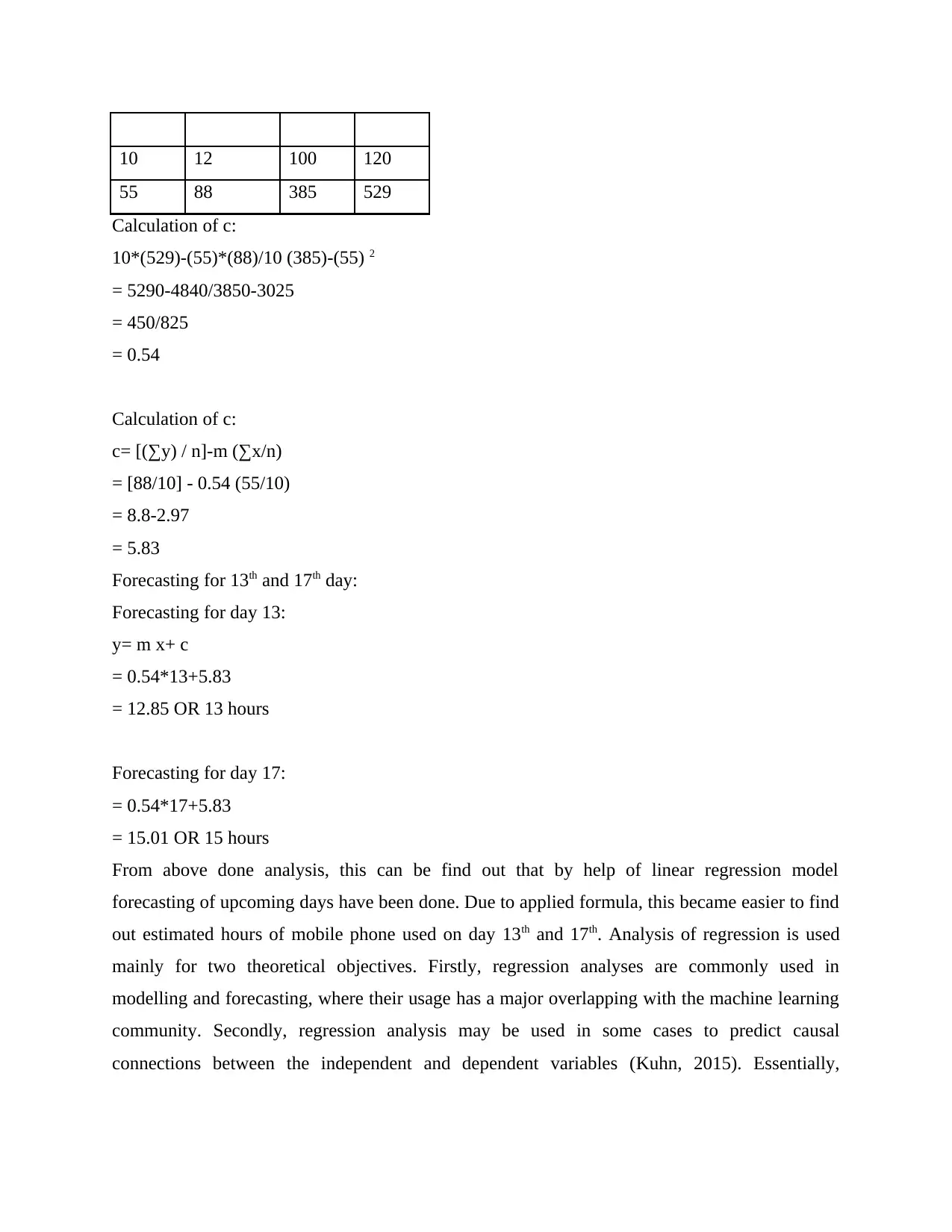
10 12 100 120
55 88 385 529
Calculation of c:
10*(529)-(55)*(88)/10 (385)-(55) 2
= 5290-4840/3850-3025
= 450/825
= 0.54
Calculation of c:
c= [(∑y) / n]-m (∑x/n)
= [88/10] - 0.54 (55/10)
= 8.8-2.97
= 5.83
Forecasting for 13th and 17th day:
Forecasting for day 13:
y= m x+ c
= 0.54*13+5.83
= 12.85 OR 13 hours
Forecasting for day 17:
= 0.54*17+5.83
= 15.01 OR 15 hours
From above done analysis, this can be find out that by help of linear regression model
forecasting of upcoming days have been done. Due to applied formula, this became easier to find
out estimated hours of mobile phone used on day 13th and 17th. Analysis of regression is used
mainly for two theoretical objectives. Firstly, regression analyses are commonly used in
modelling and forecasting, where their usage has a major overlapping with the machine learning
community. Secondly, regression analysis may be used in some cases to predict causal
connections between the independent and dependent variables (Kuhn, 2015). Essentially,

regressions itself show only connections between a dependent variable and an independent set of
factors in a defined dataset.
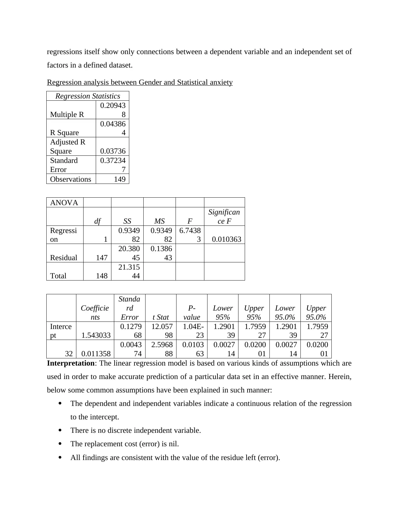
Regression analysis between Gender and Statistical anxiety
Regression Statistics
Multiple R
0.20943
8
R Square
0.04386
4
Adjusted R
Square 0.03736
Standard
Error
0.37234
7
Observations 149
ANOVA
df SS MS F
Significan
ce F
Regressi
on 1
0.9349
82
0.9349
82
6.7438
3 0.010363
Residual 147
20.380
45
0.1386
43
Total 148
21.315
44
Coefficie
nts
Standa
rd
Error t Stat
P-
value
Lower
95%
Upper
95%
Lower
95.0%
Upper
95.0%
Interce
pt 1.543033
0.1279
68
12.057
98
1.04E-
23
1.2901
39
1.7959
27
1.2901
39
1.7959
27
32 0.011358
0.0043
74
2.5968
88
0.0103
63
0.0027
14
0.0200
01
0.0027
14
0.0200
01
Interpretation: The linear regression model is based on various kinds of assumptions which are
used in order to make accurate prediction of a particular data set in an effective manner. Herein,
below some common assumptions have been explained in such manner:
 The dependent and independent variables indicate a continuous relation of the regression
to the intercept.
 There is no discrete independent variable.
 The replacement cost (error) is nil.
 All findings are consistent with the value of the residue left (error).

 These results may not have a correlation with the importance of the remaining (error).
 The residual (error) values are distributed in a typical way.
Along with the linear regression model, another key model under regression analysis is multiple
linear regressions. Linear regression is a linear method in statistical data to model the relevance
between a scalar reaction and one or more independent variable. A simple linear regression is
referred to as a descriptive component. The method is called multiple linear regressions with
more than one explaining component. Multiple linear regression models are fairly identical to the
single linear analysis, other than that the study includes more different factors. The multiple
linear regression statistical models are:
Y = b0+b1*x1+b2*x2……
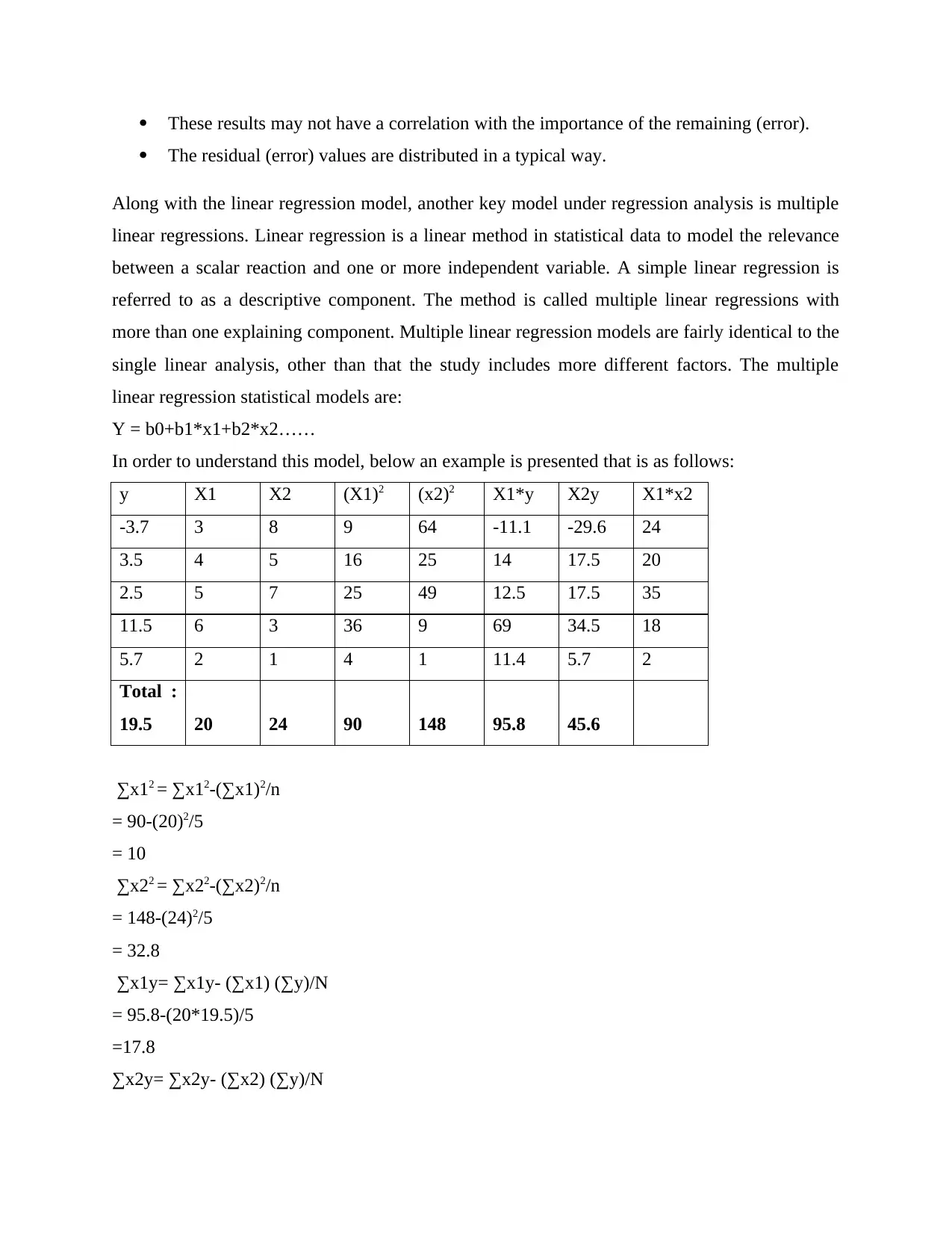
In order to understand this model, below an example is presented that is as follows:
y X1 X2 (X1)2 (x2)2 X1*y X2y X1*x2
-3.7 3 8 9 64 -11.1 -29.6 24
3.5 4 5 16 25 14 17.5 20
2.5 5 7 25 49 12.5 17.5 35
11.5 6 3 36 9 69 34.5 18
5.7 2 1 4 1 11.4 5.7 2
Total :
19.5 20 24 90 148 95.8 45.6
∑x12 = ∑x12-(∑x1)2/n
= 90-(20)2/5
= 10
∑x22 = ∑x22-(∑x2)2/n
= 148-(24)2/5
= 32.8
∑x1y= ∑x1y- (∑x1) (∑y)/N
= 95.8-(20*19.5)/5
=17.8
∑x2y= ∑x2y- (∑x2) (∑y)/N

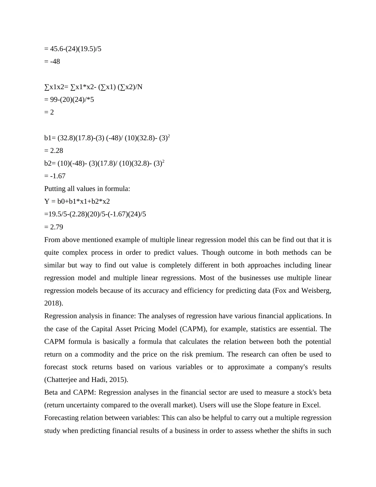
= 45.6-(24)(19.5)/5
= -48
∑x1x2= ∑x1*x2- (∑x1) (∑x2)/N
= 99-(20)(24)/*5
= 2
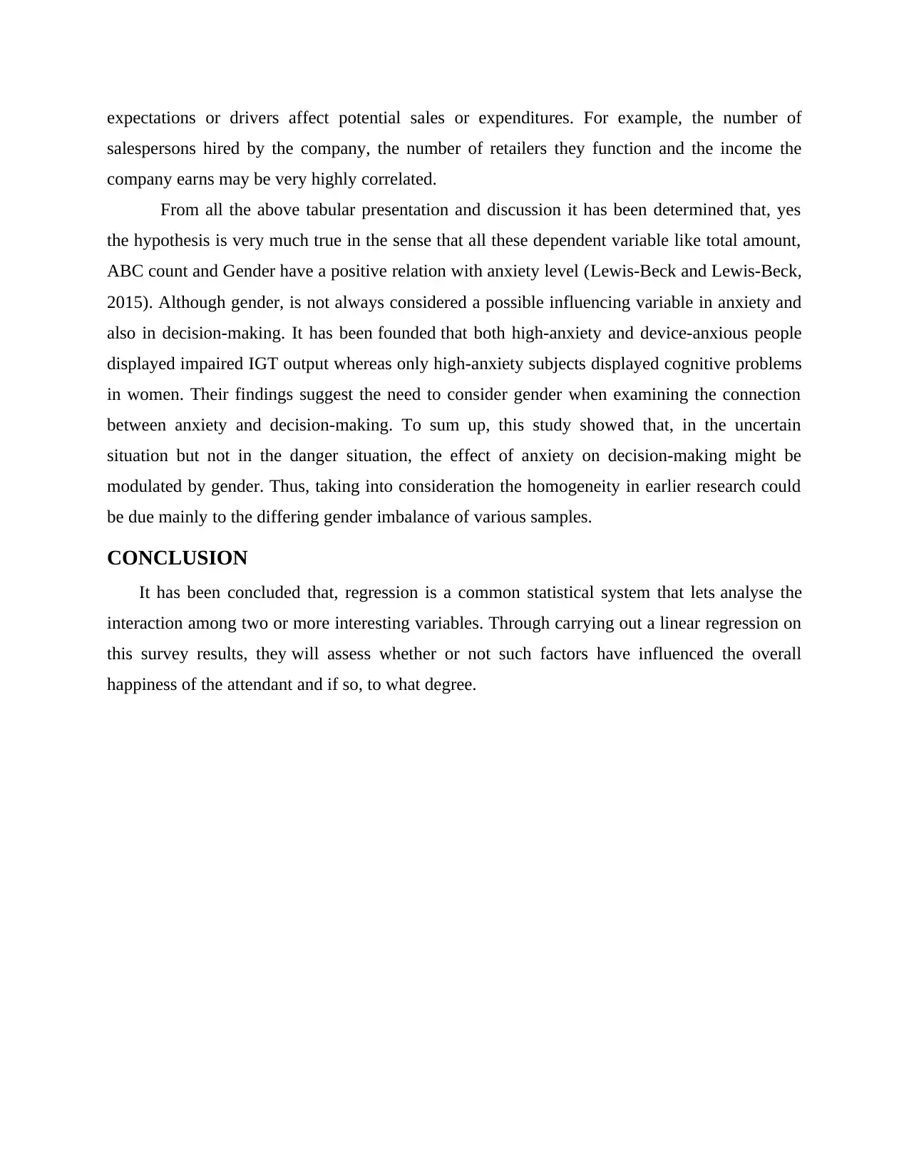
b1= (32.8)(17.8)-(3) (-48)/ (10)(32.8)- (3)2
= 2.28
b2= (10)(-48)- (3)(17.8)/ (10)(32.8)- (3)2
= -1.67
Putting all values in formula:
Y = b0+b1*x1+b2*x2
=19.5/5-(2.28)(20)/5-(-1.67)(24)/5
= 2.79
From above mentioned example of multiple linear regression model this can be find out that it is
quite complex process in order to predict values. Though outcome in both methods can be
similar but way to find out value is completely different in both approaches including linear
regression model and multiple linear regressions. Most of the businesses use multiple linear
regression models because of its accuracy and efficiency for predicting data (Fox and Weisberg,
2018).
Regression analysis in finance: The analyses of regression have various financial applications. In
the case of the Capital Asset Pricing Model (CAPM), for example, statistics are essential. The
CAPM formula is basically a formula that calculates the relation between both the potential
return on a commodity and the price on the risk premium. The research can often be used to
forecast stock returns based on various variables or to approximate a company's results
(Chatterjee and Hadi, 2015).
Beta and CAPM: Regression analyses in the financial sector are used to measure a stock's beta
(return uncertainty compared to the overall market). Users will use the Slope feature in Excel.
Forecasting relation between variables: This can also be helpful to carry out a multiple regression
study when predicting financial results of a business in order to assess whether the shifts in such

expectations or drivers affect potential sales or expenditures. For example, the number of
salespersons hired by the company, the number of retailers they function and the income the
company earns may be very highly correlated.
From all the above tabular presentation and discussion it has been determined that, yes
the hypothesis is very much true in the sense that all these dependent variable like total amount,
ABC count and Gender have a positive relation with anxiety level (Lewis-Beck and Lewis-Beck,
2015). Although gender, is not always considered a possible influencing variable in anxiety and
also in decision-making. It has been founded that both high-anxiety and device-anxious people
displayed impaired IGT output whereas only high-anxiety subjects displayed cognitive problems
in women. Their findings suggest the need to consider gender when examining the connection
between anxiety and decision-making. To sum up, this study showed that, in the uncertain
situation but not in the danger situation, the effect of anxiety on decision-making might be
modulated by gender. Thus, taking into consideration the homogeneity in earlier research could
be due mainly to the differing gender imbalance of various samples.
CONCLUSION
It has been concluded that, regression is a common statistical system that lets analyse the
interaction among two or more interesting variables. Through carrying out a linear regression on
this survey results, they will assess whether or not such factors have influenced the overall
happiness of the attendant and if so, to what degree.

REFERENCES
Books and Journals
Chatterjee, S. and Hadi, A. S., 2015. Regression analysis by example. John Wiley & Sons.
Fox, J. and Weisberg, S., 2018. An R companion to applied regression. Sage publications.
Fox, J., 2015. Applied regression analysis and generalized linear models. Sage Publications.
Kuhn, M., 2015. Caret: classification and regression training. ascl, pp.ascl-1505.
Lewis-Beck, C. and Lewis-Beck, M., 2015. Applied regression: An introduction (Vol. 22). Sage
publications.
Morris, J. S., 2015. Functional regression. Annual Review of Statistics and Its Application, 2,
pp.321-359.