Study of Life Expectancy in Australia and New Zealand

This study analyzes the life expectancy in Australia and New Zealand and its comparison with other East Asia and Pacific countries. It also studies the relationship between life expectancy at birth and health expenditure per capita (current US$) and Death rate, crude (per 1,000 people). We collected the data from World Bank. Useful for demographers, researchers and academicians.

Study of Life Expectancy in Australia and New Zealand
Author Name: Student Name

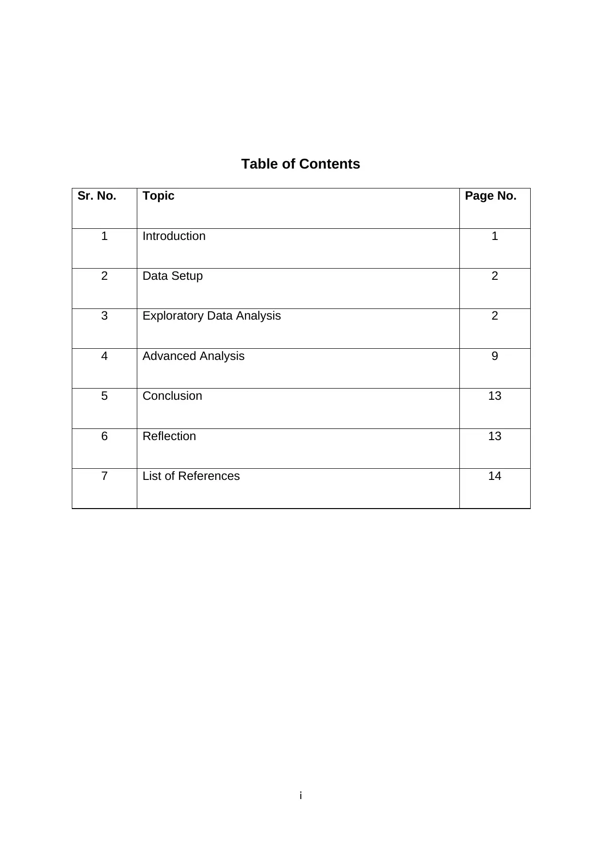
Table of Contents
Sr. No. Topic Page No.
1 Introduction 1
2 Data Setup 2
3 Exploratory Data Analysis 2
4 Advanced Analysis 9
5 Conclusion 13
6 Reflection 13
7 List of References 14
i

Study of Life Expectancy in Australia and New Zealand
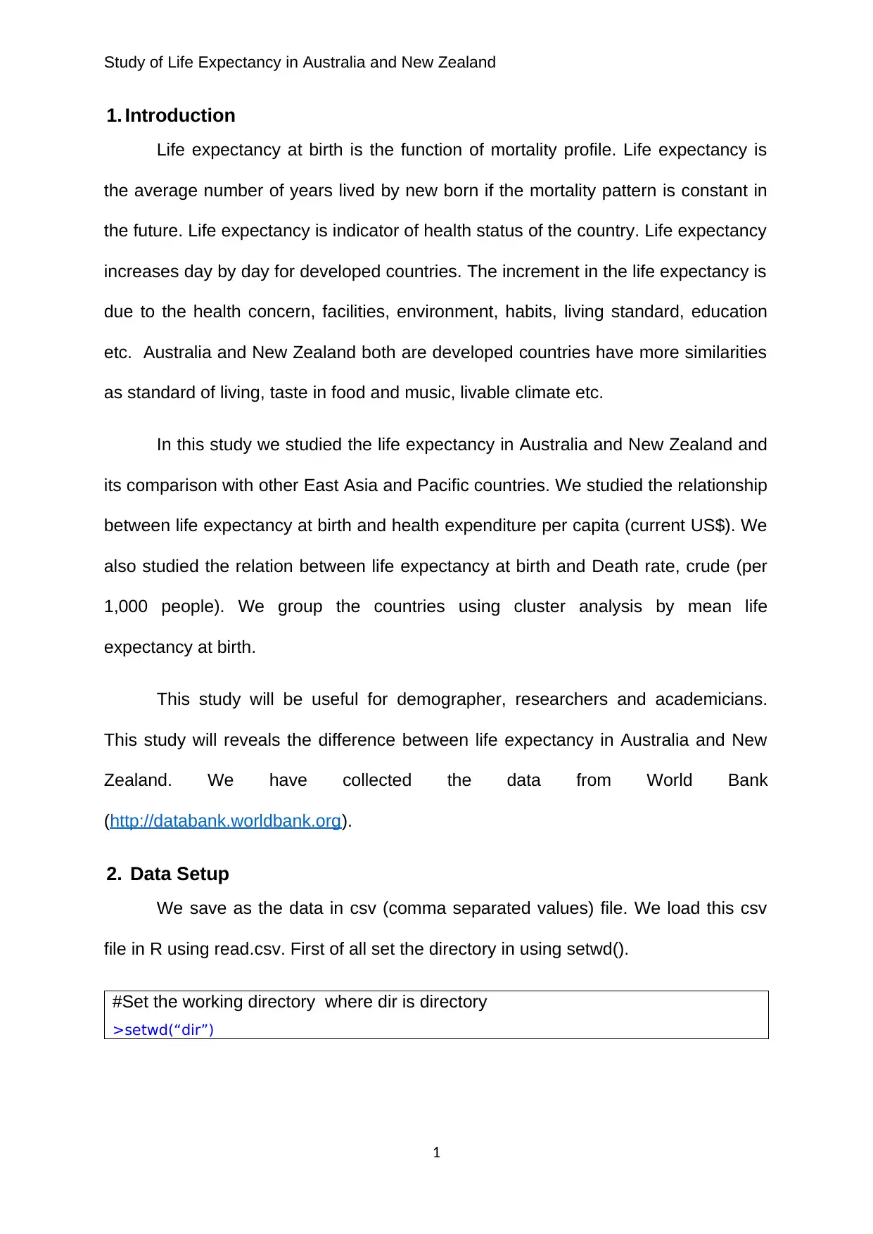
1. Introduction
Life expectancy at birth is the function of mortality profile. Life expectancy is
the average number of years lived by new born if the mortality pattern is constant in
the future. Life expectancy is indicator of health status of the country. Life expectancy
increases day by day for developed countries. The increment in the life expectancy is
due to the health concern, facilities, environment, habits, living standard, education
etc. Australia and New Zealand both are developed countries have more similarities
as standard of living, taste in food and music, livable climate etc.
In this study we studied the life expectancy in Australia and New Zealand and
its comparison with other East Asia and Pacific countries. We studied the relationship
between life expectancy at birth and health expenditure per capita (current US$). We
also studied the relation between life expectancy at birth and Death rate, crude (per
1,000 people). We group the countries using cluster analysis by mean life
expectancy at birth.
This study will be useful for demographer, researchers and academicians.
This study will reveals the difference between life expectancy in Australia and New
Zealand. We have collected the data from World Bank
(http://databank.worldbank.org).
2. Data Setup
We save as the data in csv (comma separated values) file. We load this csv
file in R using read.csv. First of all set the directory in using setwd().
#Set the working directory where dir is directory
>setwd(“dir”)
1

Study of Life Expectancy in Australia and New Zealand
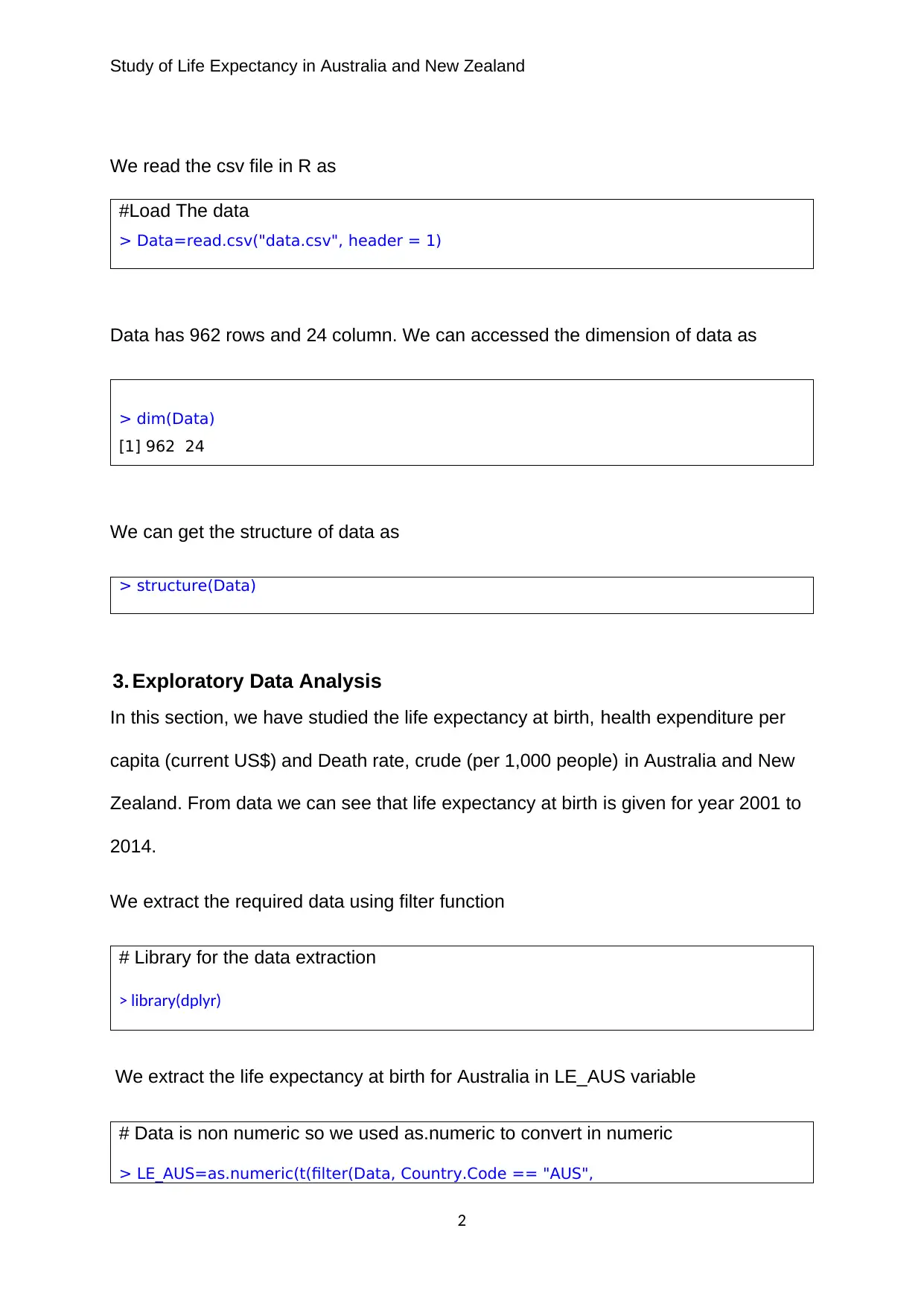
We read the csv file in R as
#Load The data
> Data=read.csv("data.csv", header = 1)
Data has 962 rows and 24 column. We can accessed the dimension of data as
> dim(Data)
[1] 962 24
We can get the structure of data as
> structure(Data)
3. Exploratory Data Analysis
In this section, we have studied the life expectancy at birth, health expenditure per
capita (current US$) and Death rate, crude (per 1,000 people) in Australia and New
Zealand. From data we can see that life expectancy at birth is given for year 2001 to
2014.
We extract the required data using filter function
# Library for the data extraction
> library(dplyr)
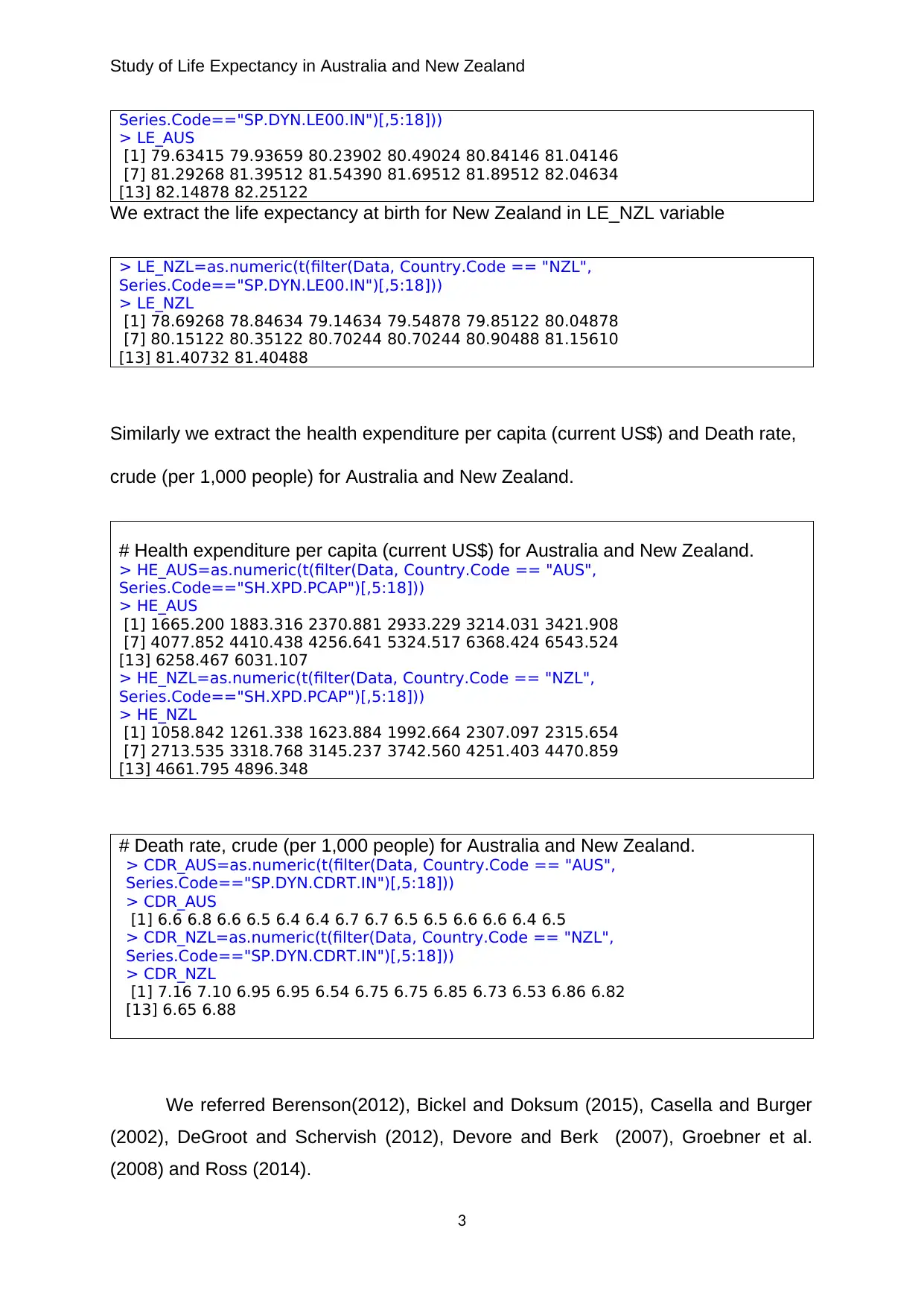
We extract the life expectancy at birth for Australia in LE_AUS variable
# Data is non numeric so we used as.numeric to convert in numeric
> LE_AUS=as.numeric(t(filter(Data, Country.Code == "AUS",
2

Study of Life Expectancy in Australia and New Zealand
Series.Code=="SP.DYN.LE00.IN")[,5:18]))
> LE_AUS
[1] 79.63415 79.93659 80.23902 80.49024 80.84146 81.04146
[7] 81.29268 81.39512 81.54390 81.69512 81.89512 82.04634
[13] 82.14878 82.25122
We extract the life expectancy at birth for New Zealand in LE_NZL variable
> LE_NZL=as.numeric(t(filter(Data, Country.Code == "NZL",
Series.Code=="SP.DYN.LE00.IN")[,5:18]))
> LE_NZL
[1] 78.69268 78.84634 79.14634 79.54878 79.85122 80.04878
[7] 80.15122 80.35122 80.70244 80.70244 80.90488 81.15610
[13] 81.40732 81.40488
Similarly we extract the health expenditure per capita (current US$) and Death rate,
crude (per 1,000 people) for Australia and New Zealand.
# Health expenditure per capita (current US$) for Australia and New Zealand.
> HE_AUS=as.numeric(t(filter(Data, Country.Code == "AUS",
Series.Code=="SH.XPD.PCAP")[,5:18]))
> HE_AUS
[1] 1665.200 1883.316 2370.881 2933.229 3214.031 3421.908
[7] 4077.852 4410.438 4256.641 5324.517 6368.424 6543.524
[13] 6258.467 6031.107
> HE_NZL=as.numeric(t(filter(Data, Country.Code == "NZL",
Series.Code=="SH.XPD.PCAP")[,5:18]))
> HE_NZL
[1] 1058.842 1261.338 1623.884 1992.664 2307.097 2315.654
[7] 2713.535 3318.768 3145.237 3742.560 4251.403 4470.859
[13] 4661.795 4896.348
# Death rate, crude (per 1,000 people) for Australia and New Zealand.
> CDR_AUS=as.numeric(t(filter(Data, Country.Code == "AUS",
Series.Code=="SP.DYN.CDRT.IN")[,5:18]))
> CDR_AUS
[1] 6.6 6.8 6.6 6.5 6.4 6.4 6.7 6.7 6.5 6.5 6.6 6.6 6.4 6.5
> CDR_NZL=as.numeric(t(filter(Data, Country.Code == "NZL",
Series.Code=="SP.DYN.CDRT.IN")[,5:18]))
> CDR_NZL
[1] 7.16 7.10 6.95 6.95 6.54 6.75 6.75 6.85 6.73 6.53 6.86 6.82
[13] 6.65 6.88
We referred Berenson(2012), Bickel and Doksum (2015), Casella and Burger
(2002), DeGroot and Schervish (2012), Devore and Berk (2007), Groebner et al.
(2008) and Ross (2014).
3

Study of Life Expectancy in Australia and New Zealand
One Variable Analysis:
Here we obtain the summary statistics of life expectancy at birth, Health
expenditure per capita (current US$) and Death rate, crude (per 1,000 people) for
Australia and New Zealand.
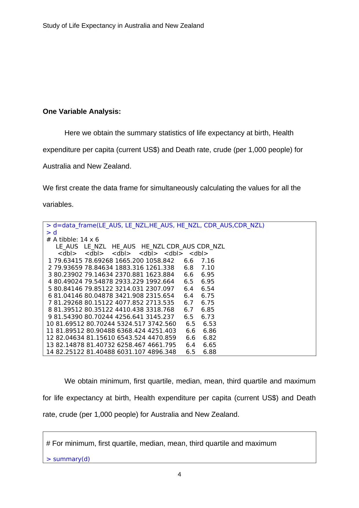
We first create the data frame for simultaneously calculating the values for all the
variables.
> d=data_frame(LE_AUS, LE_NZL,HE_AUS, HE_NZL, CDR_AUS,CDR_NZL)
> d
# A tibble: 14 x 6
LE_AUS LE_NZL HE_AUS HE_NZL CDR_AUS CDR_NZL
<dbl> <dbl> <dbl> <dbl> <dbl> <dbl>
1 79.63415 78.69268 1665.200 1058.842 6.6 7.16
2 79.93659 78.84634 1883.316 1261.338 6.8 7.10
3 80.23902 79.14634 2370.881 1623.884 6.6 6.95
4 80.49024 79.54878 2933.229 1992.664 6.5 6.95
5 80.84146 79.85122 3214.031 2307.097 6.4 6.54
6 81.04146 80.04878 3421.908 2315.654 6.4 6.75
7 81.29268 80.15122 4077.852 2713.535 6.7 6.75
8 81.39512 80.35122 4410.438 3318.768 6.7 6.85
9 81.54390 80.70244 4256.641 3145.237 6.5 6.73
10 81.69512 80.70244 5324.517 3742.560 6.5 6.53
11 81.89512 80.90488 6368.424 4251.403 6.6 6.86
12 82.04634 81.15610 6543.524 4470.859 6.6 6.82
13 82.14878 81.40732 6258.467 4661.795 6.4 6.65
14 82.25122 81.40488 6031.107 4896.348 6.5 6.88
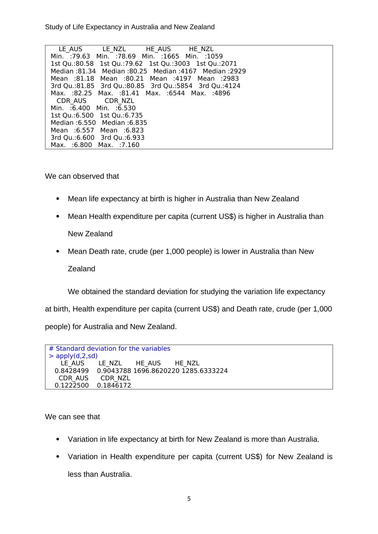
We obtain minimum, first quartile, median, mean, third quartile and maximum
for life expectancy at birth, Health expenditure per capita (current US$) and Death
rate, crude (per 1,000 people) for Australia and New Zealand.
# For minimum, first quartile, median, mean, third quartile and maximum
> summary(d)
4

Study of Life Expectancy in Australia and New Zealand
LE_AUS LE_NZL HE_AUS HE_NZL
Min. :79.63 Min. :78.69 Min. :1665 Min. :1059
1st Qu.:80.58 1st Qu.:79.62 1st Qu.:3003 1st Qu.:2071
Median :81.34 Median :80.25 Median :4167 Median :2929
Mean :81.18 Mean :80.21 Mean :4197 Mean :2983
3rd Qu.:81.85 3rd Qu.:80.85 3rd Qu.:5854 3rd Qu.:4124
Max. :82.25 Max. :81.41 Max. :6544 Max. :4896
CDR_AUS CDR_NZL
Min. :6.400 Min. :6.530
1st Qu.:6.500 1st Qu.:6.735
Median :6.550 Median :6.835
Mean :6.557 Mean :6.823
3rd Qu.:6.600 3rd Qu.:6.933
Max. :6.800 Max. :7.160
We can observed that
 Mean life expectancy at birth is higher in Australia than New Zealand
 Mean Health expenditure per capita (current US$) is higher in Australia than
New Zealand
 Mean Death rate, crude (per 1,000 people) is lower in Australia than New
Zealand
We obtained the standard deviation for studying the variation life expectancy
at birth, Health expenditure per capita (current US$) and Death rate, crude (per 1,000
people) for Australia and New Zealand.
# Standard deviation for the variables
> apply(d,2,sd)
LE_AUS LE_NZL HE_AUS HE_NZL
0.8428499 0.9043788 1696.8620220 1285.6333224
CDR_AUS CDR_NZL
0.1222500 0.1846172
We can see that
 Variation in life expectancy at birth for New Zealand is more than Australia.
 Variation in Health expenditure per capita (current US$) for New Zealand is
less than Australia.
5

Study of Life Expectancy in Australia and New Zealand
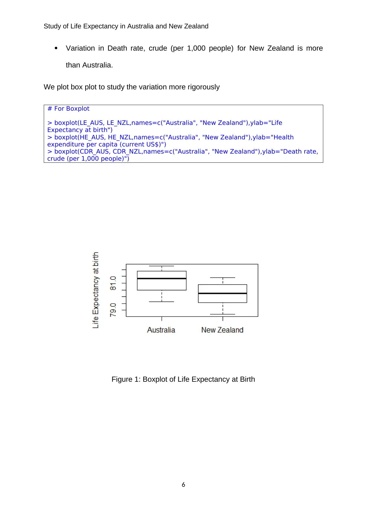
 Variation in Death rate, crude (per 1,000 people) for New Zealand is more
than Australia.
We plot box plot to study the variation more rigorously
# For Boxplot
> boxplot(LE_AUS, LE_NZL,names=c("Australia", "New Zealand"),ylab="Life
Expectancy at birth")
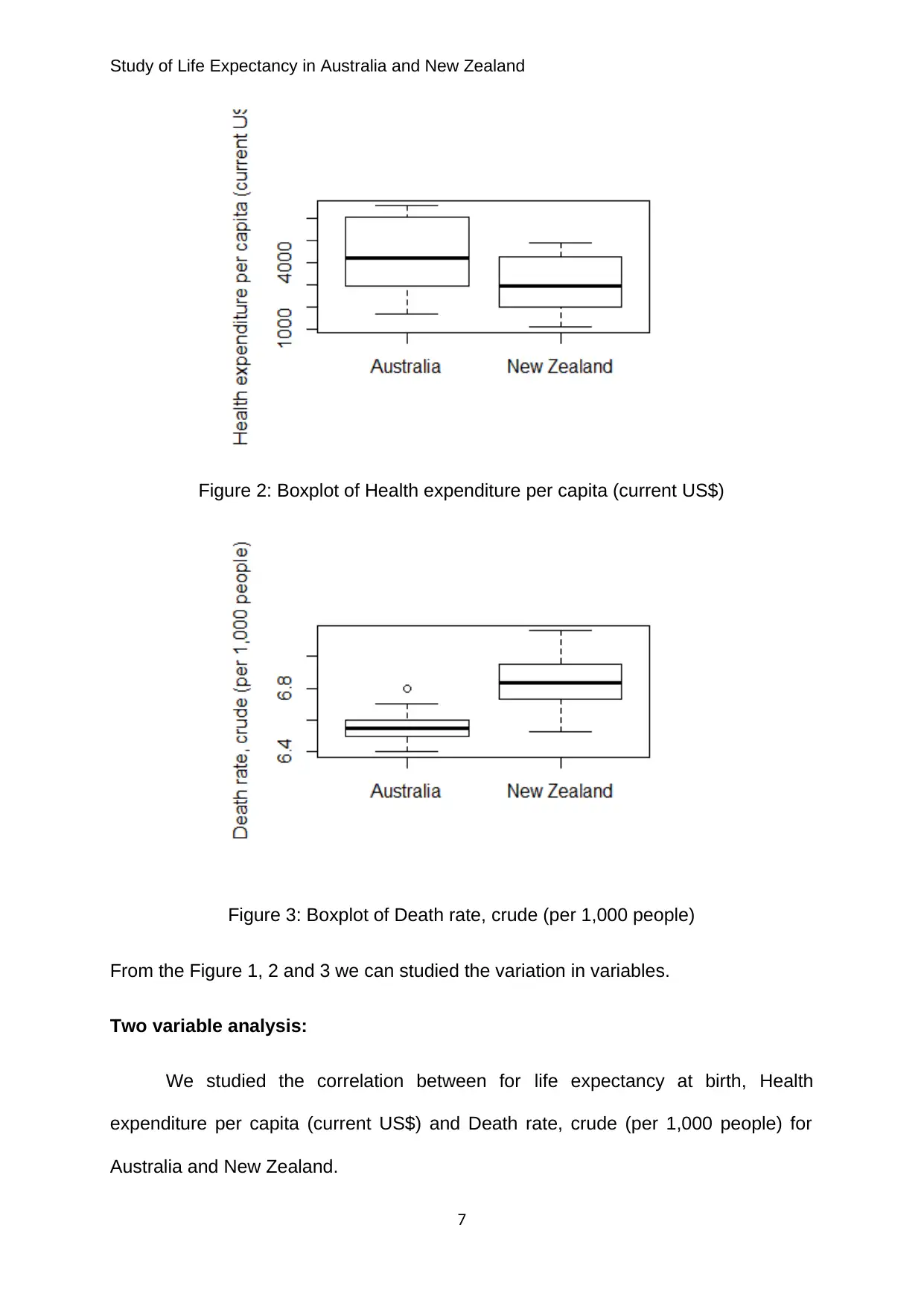
> boxplot(HE_AUS, HE_NZL,names=c("Australia", "New Zealand"),ylab="Health
expenditure per capita (current US$)")
> boxplot(CDR_AUS, CDR_NZL,names=c("Australia", "New Zealand"),ylab="Death rate,
crude (per 1,000 people)")
Figure 1: Boxplot of Life Expectancy at Birth
6

Study of Life Expectancy in Australia and New Zealand
Figure 2: Boxplot of Health expenditure per capita (current US$)
Figure 3: Boxplot of Death rate, crude (per 1,000 people)
From the Figure 1, 2 and 3 we can studied the variation in variables.
Two variable analysis:
We studied the correlation between for life expectancy at birth, Health
expenditure per capita (current US$) and Death rate, crude (per 1,000 people) for
Australia and New Zealand.
7

Study of Life Expectancy in Australia and New Zealand
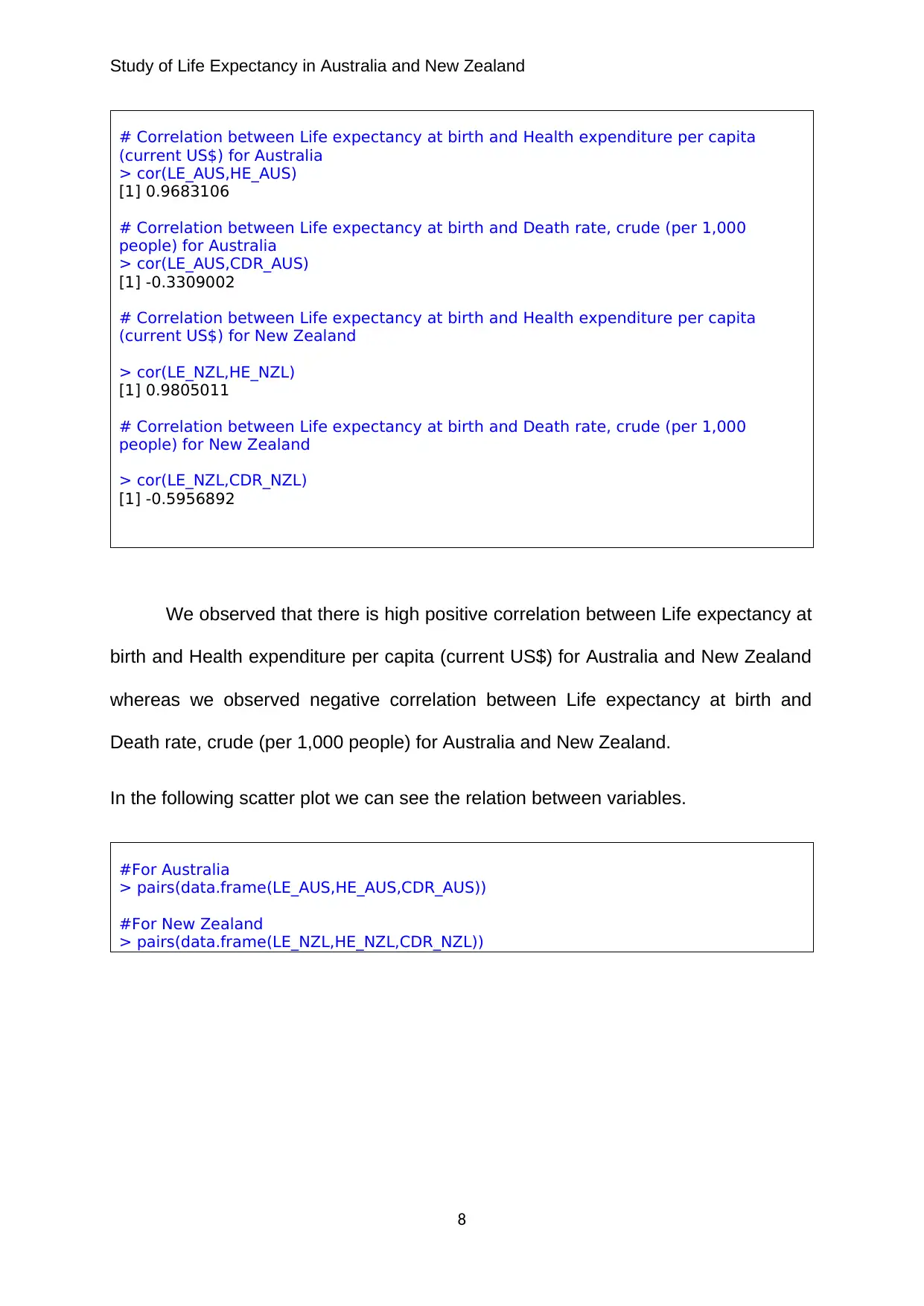
# Correlation between Life expectancy at birth and Health expenditure per capita
(current US$) for Australia
> cor(LE_AUS,HE_AUS)
[1] 0.9683106
# Correlation between Life expectancy at birth and Death rate, crude (per 1,000
people) for Australia
> cor(LE_AUS,CDR_AUS)
[1] -0.3309002
# Correlation between Life expectancy at birth and Health expenditure per capita
(current US$) for New Zealand
> cor(LE_NZL,HE_NZL)
[1] 0.9805011
# Correlation between Life expectancy at birth and Death rate, crude (per 1,000
people) for New Zealand
> cor(LE_NZL,CDR_NZL)
[1] -0.5956892
We observed that there is high positive correlation between Life expectancy at
birth and Health expenditure per capita (current US$) for Australia and New Zealand
whereas we observed negative correlation between Life expectancy at birth and
Death rate, crude (per 1,000 people) for Australia and New Zealand.
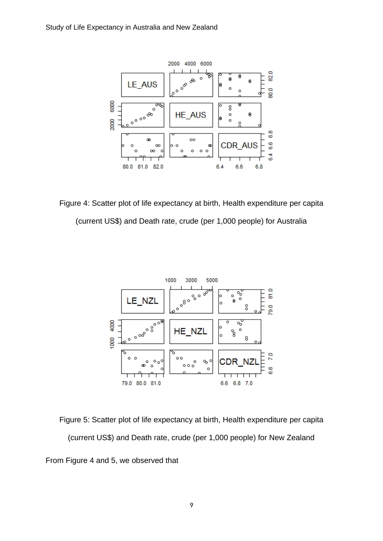
In the following scatter plot we can see the relation between variables.
#For Australia
> pairs(data.frame(LE_AUS,HE_AUS,CDR_AUS))
#For New Zealand
> pairs(data.frame(LE_NZL,HE_NZL,CDR_NZL))
8

Study of Life Expectancy in Australia and New Zealand
Figure 4: Scatter plot of life expectancy at birth, Health expenditure per capita
(current US$) and Death rate, crude (per 1,000 people) for Australia
Figure 5: Scatter plot of life expectancy at birth, Health expenditure per capita
(current US$) and Death rate, crude (per 1,000 people) for New Zealand
From Figure 4 and 5, we observed that
9

Study of Life Expectancy in Australia and New Zealand
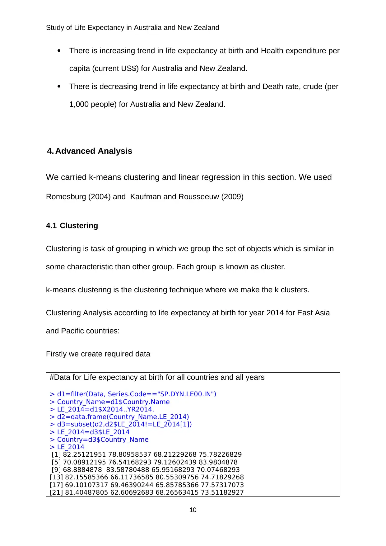
 There is increasing trend in life expectancy at birth and Health expenditure per
capita (current US$) for Australia and New Zealand.
 There is decreasing trend in life expectancy at birth and Death rate, crude (per
1,000 people) for Australia and New Zealand.
4. Advanced Analysis
We carried k-means clustering and linear regression in this section. We used
Romesburg (2004) and Kaufman and Rousseeuw (2009)
4.1 Clustering
Clustering is task of grouping in which we group the set of objects which is similar in
some characteristic than other group. Each group is known as cluster.
k-means clustering is the clustering technique where we make the k clusters.
Clustering Analysis according to life expectancy at birth for year 2014 for East Asia
and Pacific countries:
Firstly we create required data
#Data for Life expectancy at birth for all countries and all years
> d1=filter(Data, Series.Code=="SP.DYN.LE00.IN")
> Country_Name=d1$Country.Name
> LE_2014=d1$X2014..YR2014.
> d2=data.frame(Country_Name,LE_2014)
> d3=subset(d2,d2$LE_2014!=LE_2014[1])
> LE_2014=d3$LE_2014
> Country=d3$Country_Name
> LE_2014
[1] 82.25121951 78.80958537 68.21229268 75.78226829
[5] 70.08912195 76.54168293 79.12602439 83.9804878
[9] 68.8884878 83.58780488 65.95168293 70.07468293
[13] 82.15585366 66.11736585 80.55309756 74.71829268
[17] 69.10107317 69.46390244 65.85785366 77.57317073
[21] 81.40487805 62.60692683 68.26563415 73.51182927
10

Study of Life Expectancy in Australia and New Zealand
[25] 82.64634146 67.93080488 74.42202439 68.25914634
[29] 72.79219512 71.91831707 75.62912195
> Country=d3$Country_Name
> Country
[1] Australia
[2] Brunei Darussalam
[3] Cambodia
[4] China
[5] Fiji
[6] French Polynesia
[7] Guam
[8] Hong Kong SAR, China
[9] Indonesia
[10] Japan
[11] Kiribati
[12] Korea, Dem. People’s Rep.
[13] Korea, Rep.
[14] Lao PDR
[15] Macao SAR, China
[16] Malaysia
[17] Micronesia, Fed. Sts.
[18] Mongolia
[19] Myanmar
[20] New Caledonia
[21] New Zealand
[22] Papua New Guinea
[23] Philippines
[24] Samoa
[25] Singapore
[26] Solomon Islands
[27] Thailand
[28] Timor-Leste
[29] Tonga
[30] Vanuatu
[31] Vietnam
We group the data in 3 groups, we used k-means clustering
> kmeans(LE_2014,3)
K-means clustering with 3 clusters of sizes 9, 9, 13
Cluster means:
[,1]
1 74.76543
2 81.61281
3 67.75531
Clustering vector:
[1] 2 2 3 1 3 1 2 2 3 2 3 3 2 3 2 1 3 3 3 1 2 3 3 1 2
[26] 3 1 3 1 1 1
Within cluster sum of squares by cluster:
[1] 26.50978 26.48555 53.63666
(between_SS / total_SS = 90.6 %)
Available components:
11

Study of Life Expectancy in Australia and New Zealand
[1] "cluster" "centers" "totss"
[4] "withinss" "tot.withinss" "betweenss"
[7] "size" "iter" "ifault"
We can group the countries using clustering vector. We can observe that
Australia and New Zealand are in second group which has high life expectancy. We
observed that about 90.6 % variation is explained by the clusters.
4.2 Linear Regression
We fit the linear regression to the life expectancy at birth by time for Australia and
New Zealand. We used Baayen (2008) and Hair et al. (1998).
Australia:
We have data of life expectancy at birth from year 2001 to 2014. We fitted the linear
regression to predict the life expectancy at birth for future.
> LE_AUS=as.numeric(t(filter(Data, Country.Code == "AUS",
Series.Code=="SP.DYN.LE00.IN")[,5:18]))
> Year=2001:2014
> dataAUS=data.frame(Year,LE_AUS)
> result=lm(LE_AUS~Year,data=dataAUS)
> summary(result)
Call:
lm(formula = LE_AUS ~ Year, data = dataAUS)
Residuals:
Min 1Q Median 3Q Max
-0.25045 -0.09935 0.01686 0.10833 0.21686
Coefficients:
Estimate Std. Error t value Pr(>|t|)
(Intercept) -3.174e+02 1.988e+01 -15.96 1.91e-09
Year 1.985e-01 9.905e-03 20.04 1.36e-10
(Intercept) ***
Year ***
---
Signif. codes:
0 ‘***’ 0.001 ‘**’ 0.01 ‘*’ 0.05 ‘.’ 0.1 ‘ ’ 1
Residual standard error: 0.1494 on 12 degrees of freedom
Multiple R-squared: 0.971, Adjusted R-squared: 0.9686
12

Study of Life Expectancy in Australia and New Zealand
F-statistic: 401.8 on 1 and 12 DF, p-value: 1.359e-10
We found that R2 is 0.971 which suggest that fitting is good. Each year brings 0.1985
more years for new born baby in Australia.
New Zealand:
We have data of life expectancy at birth from year 2001 to 2014. We fitted the linear
regression to predict the life expectancy at birth for future.
>
> LE_NZL=as.numeric(t(filter(Data, Country.Code == "NZL",
Series.Code=="SP.DYN.LE00.IN")[,5:18]))
> Year=2001:2014
> dataNZL=data.frame(Year,LE_NZL)
> result1=lm(LE_NZL~Year,data=dataNZL)
> summary(result1)
Call:
lm(formula = LE_NZL ~ Year, data = dataNZL)
Residuals:
Min 1Q Median 3Q Max
-0.195122 -0.086900 0.002895 0.080046 0.178344
Coefficients:
Estimate Std. Error t value Pr(>|t|)
(Intercept) -3.496e+02 1.727e+01 -20.25 1.21e-10
Year 2.141e-01 8.601e-03 24.89 1.07e-11
(Intercept) ***
Year ***
---
Signif. codes:
0 ‘***’ 0.001 ‘**’ 0.01 ‘*’ 0.05 ‘.’ 0.1 ‘ ’ 1
Residual standard error: 0.1297 on 12 degrees of freedom
Multiple R-squared: 0.981, Adjusted R-squared: 0.9794
F-statistic: 619.8 on 1 and 12 DF, p-value: 1.068e-11
We found that R2 is 0.981 which suggest that fitting is good. Each year brings 0.214
more years for new born baby in New Zealand.
5. Conclusion
13

Study of Life Expectancy in Australia and New Zealand
We can observed that mean life expectancy at birth is higher in Australia than New
Zealand, mean Health expenditure per capita (current US$) is higher in Australia
than New Zealand and mean Death rate, crude (per 1,000 people) is lower in
Australia than New Zealand
We observed that there is high positive correlation between Life expectancy at birth
and Health expenditure per capita (current US$) for Australia and New Zealand
whereas we observed negative correlation between Life expectancy at birth and
Death rate, crude (per 1,000 people) for Australia and New Zealand.
We can observe that Australia and New Zealand are in second group which has high
life expectancy. We observed that about 90.6 % variation is explained by the
clusters.
Each year brings 0.1985 more years for new born baby in Australia. Each year brings
0.214 more years for new born baby in New Zealand.
6. Reflection
Data filter and sub selection of variables of interest is main problem in this
analysis we solve this problem by using filter function define in dplyr library. After
getting the desired data, it was interesting to work on the given problem under study.
By doing this study, we got the confidence on the data analysis of big data.
List of References
Berenson, M., Levine, D., Szabat, K.A. and Krehbiel, T.C., 2012. Basic business
statistics: Concepts and applications. Pearson higher education AU.
14

Study of Life Expectancy in Australia and New Zealand
Bickel, P.J. and Doksum, K.A., 2015. Mathematical statistics: basic ideas and
selected topics, volume I (Vol. 117). CRC Press.
Casella, G. and Berger, R.L., 2002. Statistical inference (Vol. 2). Pacific Grove, CA:
Duxbury.
DeGroot, M.H. and Schervish, M.J., 2012. Probability and statistics. Pearson
Education.
Devore, J.L. and Berk, K.N., 2007. Modern mathematical statistics with applications.
Cengage Learning.
Groebner, D.F., Shannon, P.W., Fry, P.C. and Smith, K.D., 2008. Business statistics.
Pearson Education.
Ross, S.M., 2014. Introduction to probability models. Academic press.
Baayen, R.H., 2008. Analyzing linguistic data: A practical introduction to statistics
using R. Cambridge University Press.
Kaufman, L. and Rousseeuw, P.J., 2009. Finding groups in data: an introduction to
cluster analysis (Vol. 344). John Wiley & Sons.
Romesburg, C., 2004. Cluster analysis for researchers. Lulu. com.
Hair, J.F., Black, W.C., Babin, B.J., Anderson, R.E. and Tatham, R.L.,
1998. Multivariate data analysis (Vol. 5, No. 3, pp. 207-219). Upper Saddle
River, NJ: Prentice hall.
15