Linear Algebra, Calculus and Probability Theory Solutions
VerifiedAdded on 2022/11/19
|12
|1439
|328
AI Summary
Get solutions for Linear Algebra, Calculus and Probability Theory problems. Topics include fields, vector spaces, bases, chain rule, variance, probability density function and more.
Contribute Materials
Your contribution can guide someone’s learning journey. Share your
documents today.
LINEAR ALGEBRA
Solutions
a.
since the matrix has fewer rows than columns it therefore means that the rank must be equal to the
number of rows .Row one is dependent on row 2 and can be derived from the scalar multiple of 2
meaning that there are no linearly dependent number of rows and the rank of the matrix is zero
2R1=R2
2(2)=α; α=4
For the Determinant of the matrix to be evaluated it must be a square matrix and therefore since it is 2
by 6 matrix
The same case is for the eigen values which can only be evaluated only for a square matrix
b. Since the number of rows are fewer than the number of columns then the maximum rank of the
matrix must be equal to the number of rows. Looking at the rows more closely it appears that the rows
are linearly independent of each other therefore the rank of the matrix is 3
The determinant of the matrix cannot be evaluated since it is not a square matrix 3×4 matrix
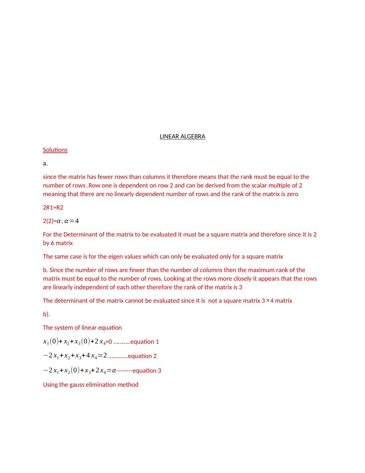
b).
The system of linear equation
x1 (0)+ x2 + x3 (0)+2 x4=0 ………..equation 1
−2 x1 +x2 + x3+ 4 x4 =2 ………….equation 2
−2 x1 + x2 (0)+ x3+ 2 x4 =α--------equation 3
Using the gauss elimination method
Solutions
a.
since the matrix has fewer rows than columns it therefore means that the rank must be equal to the
number of rows .Row one is dependent on row 2 and can be derived from the scalar multiple of 2
meaning that there are no linearly dependent number of rows and the rank of the matrix is zero
2R1=R2
2(2)=α; α=4
For the Determinant of the matrix to be evaluated it must be a square matrix and therefore since it is 2
by 6 matrix
The same case is for the eigen values which can only be evaluated only for a square matrix
b. Since the number of rows are fewer than the number of columns then the maximum rank of the
matrix must be equal to the number of rows. Looking at the rows more closely it appears that the rows
are linearly independent of each other therefore the rank of the matrix is 3
The determinant of the matrix cannot be evaluated since it is not a square matrix 3×4 matrix
b).
The system of linear equation
x1 (0)+ x2 + x3 (0)+2 x4=0 ………..equation 1
−2 x1 +x2 + x3+ 4 x4 =2 ………….equation 2
−2 x1 + x2 (0)+ x3+ 2 x4 =α--------equation 3
Using the gauss elimination method
Secure Best Marks with AI Grader
Need help grading? Try our AI Grader for instant feedback on your assignments.
[ x1
x2
x3
x4
]=
[ −1+x2 /2+ x3
2 + x4 /2
1−2 x4
α −2 x4 +2 x1
x4
]
[ x1
x2
x3
x4
]=
[−1
1
α
0 ]+ x1
[0
0
2
0 ]+ x2
[0.5
0
0
0 ]+ x3
[0.5
0
0
0 ]+ x4
[0.5
−2
−2
1 ]
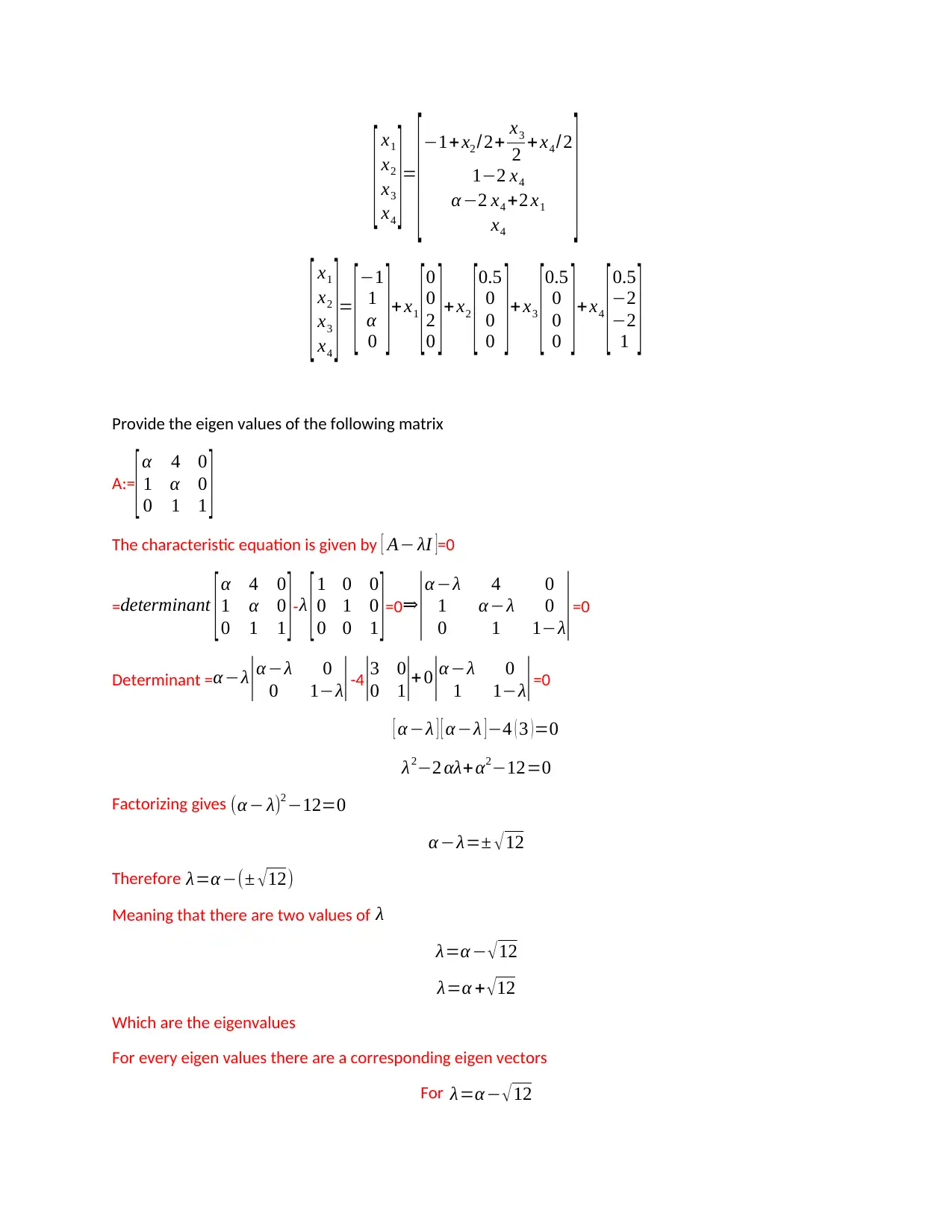
Provide the eigen values of the following matrix
A:=
[α 4 0
1 α 0
0 1 1 ]
The characteristic equation is given by [ A− λI ]=0
=determinant [α 4 0
1 α 0
0 1 1 ]-λ [1 0 0
0 1 0
0 0 1 ]=0⇒
|α −λ 4 0
1 α −λ 0
0 1 1−λ|=0
Determinant = α −λ |α −λ 0
0 1−λ|-4|3 0
0 1|+ 0 |α −λ 0
1 1−λ|=0
[ α −λ ] [ α −λ ] −4 ( 3 ) =0
λ2−2 αλ+α2−12=0
Factorizing gives (α − λ)2 −12=0
α −λ=± √12
Therefore λ=α −(± √ 12)
Meaning that there are two values of λ
λ=α − √12
λ=α + √12
Which are the eigenvalues
For every eigen values there are a corresponding eigen vectors
For λ=α− √12
x2
x3
x4
]=
[ −1+x2 /2+ x3
2 + x4 /2
1−2 x4
α −2 x4 +2 x1
x4
]
[ x1
x2
x3
x4
]=
[−1
1
α
0 ]+ x1
[0
0
2
0 ]+ x2
[0.5
0
0
0 ]+ x3
[0.5
0
0
0 ]+ x4
[0.5
−2
−2
1 ]
Provide the eigen values of the following matrix
A:=
[α 4 0
1 α 0
0 1 1 ]
The characteristic equation is given by [ A− λI ]=0
=determinant [α 4 0
1 α 0
0 1 1 ]-λ [1 0 0
0 1 0
0 0 1 ]=0⇒
|α −λ 4 0
1 α −λ 0
0 1 1−λ|=0
Determinant = α −λ |α −λ 0
0 1−λ|-4|3 0
0 1|+ 0 |α −λ 0
1 1−λ|=0
[ α −λ ] [ α −λ ] −4 ( 3 ) =0
λ2−2 αλ+α2−12=0
Factorizing gives (α − λ)2 −12=0
α −λ=± √12
Therefore λ=α −(± √ 12)
Meaning that there are two values of λ
λ=α − √12
λ=α + √12
Which are the eigenvalues
For every eigen values there are a corresponding eigen vectors
For λ=α− √12
Eigen vector corresponding to λ=α− √12
becomes
Replacing λ=α − √12 in the matrix becomes [ √12 4 0
3 √12 0
0 1 1−(α − √12) ] [x1
x2
x3 ]=
[ 0
0
0 ]
[ √12 4 0
3 √12 0
0 1 4.464−α ] [ x1
x2
x3 ]=
[0
0
0 ]
( √12 ) x1 +4 x2 =0 ⇒ x1=1.154 x2=1.154t
3 x1+ ( √12 ) x2=0 ⟹ x2=¿-0.866x1=-0.0866(1.154t)=-0.09994t
x2+ ( 4.464−α ) x3=0⇒ x3 = −1
4.464−α ; x2= −1
4.464−α t
[ x1
x2
x3 ]=
[ 1.154 t
−0.09994 t
−1
4.464−α t ] Where tϵ R
Eigen vector corresponding to eigen value λ=α + √12
is gotten by plugging in λ=α + √12 in the characteristic equation and it becomes
[ − √ 12 4 0
3 − √ 12 0
0 1 1−(α+ √ 12) ] [ x1
x2
x3 ]=
[0
0
0 ]
[− √12 4 0
3 − √12 0
0 1 −2.464−α ] [ x1
x2
x3 ]=
[ 0
0
0 ]
Converting into system of linear equations becomes
( − √ 12 ) x1 + 4 x2=0 ⇒ x1=1.154 x2=-1.154t
3 x1+ ( − √ 12 ) x2=0 ⟹ x2 =¿0.866 x1=0.0866(1.154t)=0.09994t
x2+ (−2.464−α ) x3=0 ⇒ x3= 1
2.464+ α x2= 1
2.464+α t
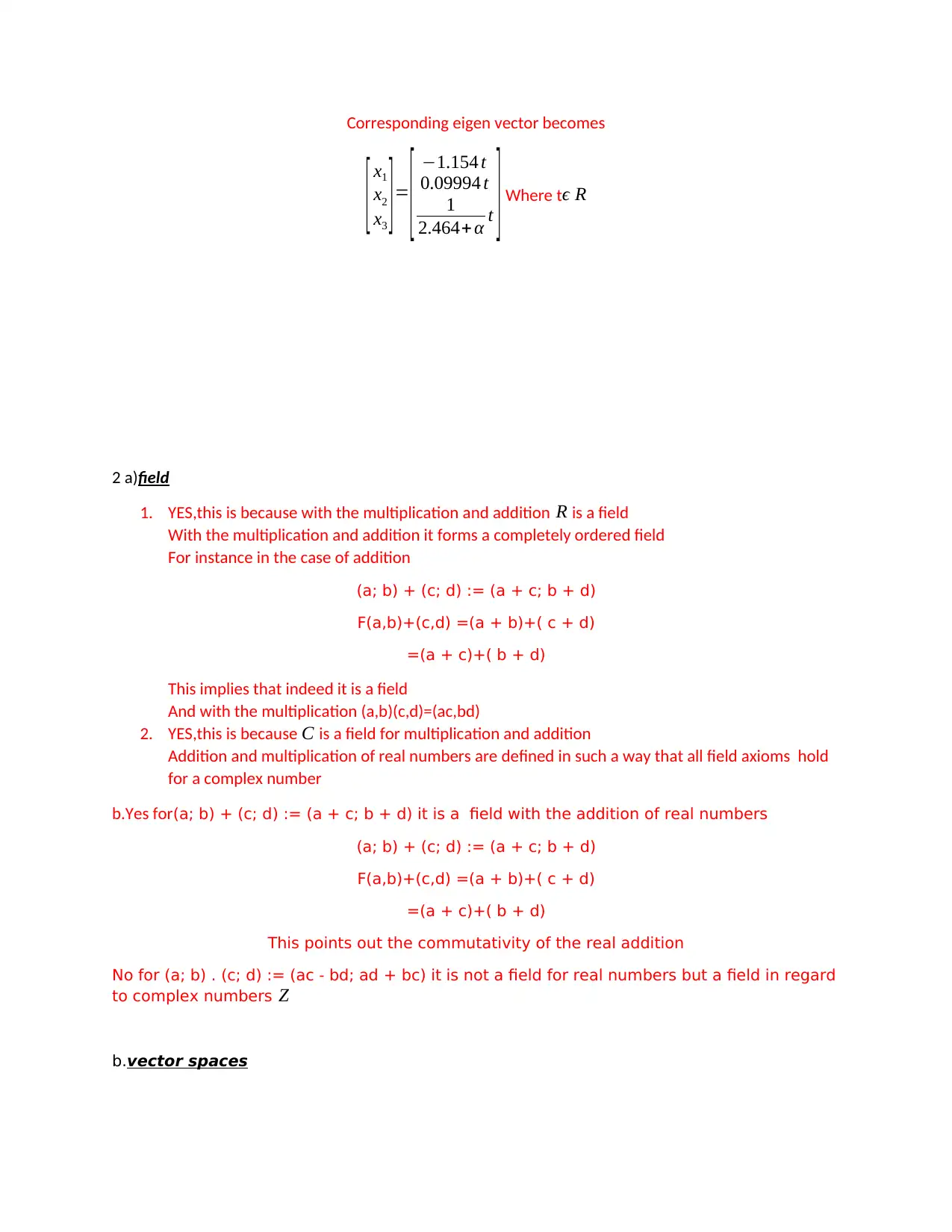
Corresponding eigen vector becomes
[ x1
x2
x3 ]=
[ −1.154 t
0.09994 t
1
2.464+ α t ] Where tϵ R
2 a)field
1. YES,this is because with the multiplication and addition R is a field
With the multiplication and addition it forms a completely ordered field
For instance in the case of addition
(a; b) + (c; d) := (a + c; b + d)
F(a,b)+(c,d) =(a + b)+( c + d)
=(a + c)+( b + d)
This implies that indeed it is a field
And with the multiplication (a,b)(c,d)=(ac,bd)
2. YES,this is because C is a field for multiplication and addition
Addition and multiplication of real numbers are defined in such a way that all field axioms hold
for a complex number
b.Yes for(a; b) + (c; d) := (a + c; b + d) it is a field with the addition of real numbers
(a; b) + (c; d) := (a + c; b + d)
F(a,b)+(c,d) =(a + b)+( c + d)
=(a + c)+( b + d)
This points out the commutativity of the real addition
No for (a; b) . (c; d) := (ac - bd; ad + bc) it is not a field for real numbers but a field in regard
to complex numbers Z
b.vector spaces
Secure Best Marks with AI Grader
Need help grading? Try our AI Grader for instant feedback on your assignments.
(i)Yes this is because vector addition as well multiplication is associative over the complex
numbers
(ii)Yes this is because for the complex numbers vector addition as well as multiplication is
associative over the real numbers hence a vector space
3. (i) Yes (a; b) + (c; d) := (a + c; b + d); (a; b); (c; d) 2 ϵ V;
(ii)Yes λ .(a; b) := ( λa; λb); λϵ R; (a; b) 2 V;
4.Yes;The RM × N where M × N is a vector field together with usual matrix addition and
multiplication
C Subspace
a. if c=0 then it is a subspace meaning that ax+by=0 For it to be a subspace ,(0,0,0) had to be in the
space and hence c=0 a=0 b=0
b. if c=0 then it is a subspace ax + by ≥c;
a and b are any real numbers ≥ 0
c.no this is because it is linearly dependent on each other
d.
A matrix for it to be a subspace it must satisfy the following conditions
1. Non emptiness
2. Closure under addition
3. Closure under scalar multiplication
Letting the matrix be
[ x 1
0 y ]
And c be 2 which is the scalar
And determining condition 3 becomes [ 2 x 2
0 2 y ]
Which is not in the first matrix meaning that
For the matrix to be a subspace then the value of aϵ Rfor it to be subspace
d.dimension
a.)Yes:α1 [ 1
0 ] +α2 [ 1
2 ] +α 3 [ 2
3 ]:α 1 , α 2 , α3 ϵ R
α1+ α2 +2 α 3
0( α¿¿ 1)+2 α2 ¿+3 α 3
The two expressions are linearly independent of each other and therefore the dimension of the matrix is
2
In order to get the basis for the set of vectors we check for 0 and 1 which forms the basis for the vector
Therefore [1
0 ] is the basis
b.) no;x ≠ 0 proving that it is not a subspace
CALCULUS
a). i
l1= lim
n →+∞
2 n3+ n−2
5 n3−n2−2
plugging∈∞ becomes anindeterminate function∧therefore there is need ¿ the|limit even
further ¿ becomethrough factorization=
lim
n →+ ∞
n3 (2+ 1
n2 − 2
n3 )
n3 (5−1
n − 2
n3 )
n3 cancels out ∈the above function∧therefore becomes
l1=
lim
n →+∞
(2+ 1
n2 − 2
n3 )
( 5− 1
n − 2
n3 )
Now plugging in ∞the limit becomes l1=
(2+ 1
∞2 − 2
∞3 )
(5− 1
∞ − 2
∞3 )
Which is l1= (2+ 0−0)
(5−0−0)= 2
5
ANSWER, l1= 2
5
ii)
l2= lim
n →+∞
(1+ 2
n−1 )
3 n
;By plugging ∞ it becomes
l2=(1+ 2
∞−1 )
3 × ∞
which implies that l2=(1+ 2
∞ )
∞
2
∞ =0
Thereforel2=(1+0)∞ ⇒ 1∞
Meaning l2=1
b.)
d
dx (3 sin (cos (log 3 x2+1
4 x5−2 ) ))
3 d
dx (sin (cos (log 3 x2+1
4 x5−2 ) ))
pull constants out of derivative
3 d
dx (cos ( log 3 x2 +1
4 x5−2 )) cos ( cos ( log 3 x2+1
4 x5−2 ) )
Chain rule: Differentiate the outside function and multiply this by the derivative of the inside
function
3 cos ( cos ( log 3 x2+1
4 x5−2 ) ) d
dx ( log 3 x2+ 1
4 x5−2 ) .(−sin ( log 3 x2 +1
4 x5−2 ))¿
simplify the product futher ¿ give
3 cos (cos (log 3 x2+1
4 x5−2 ) ) d
dx (log 3 x2+ 1
4 x5−2 )(−sin ( log 3 x2 +1
4 x5−2 )) 1
3 x2 +1
2¿ ¿ ¿
−3 cos (cos (log 3 x2+1
4 x5−2 ) )sin (log 3 x2 +1
4 x5−2 ).1 ¿ ¿
Carry down the unmodified factors of 3
Chain rule:Differentiate the outside function and multiply by the derivative of the inside
function
−3 ¿ ¿
simplifying even further through factoring out becomes
−6 cos (cos (log 3 x2 +1
2 ( 2 x5−1 ) ))sin (log 3 x2+1
2 ( 2 x5−1 ) )2 ¿ ¿
Paraphrase This Document
Need a fresh take? Get an instant paraphrase of this document with our AI Paraphraser
( 2 x5−1 ) .6 x1−(3 x2+1)¿
c).
f ( x ) =3 g2 (2 x ,−1 ,−sin2 x )
Since ∇ g ( x ) is said to be the gradient vector
f’(x)=3 g2 ¿)
f’(x)=3 g2 (2−2 cosx)
PROBABILITY THEORY
Solution
4 a
From the probability density function integrating p× ( x )= 1−x2 + x
c should give 1
This means integrating the function would give the unknown constant c
∫
0
1
1−x2 + x
c dx=1
1
c ∫
0
1
1−x2 +xdx=1
1
c [ x− x3
3 + x2
2 ] ¿ limit 0 ¿ 1 =1
1
c [ ( 1− 13
3 + 12
2 +constant of integration )−(0+constant of integration) ]=1
Therefore
c=1− 1
3 + 1
2 = 7
6
c= 7
6
b).Cumulative distribution function (cdf ) can be evaluated by getting the integral of
6
7 ∫
0
1
(1−x2+ x) dx
Integrating it becomes 6
7 [ x − x3
3 + x2
2 ] from the limit 0 to 1
6
7 [ 1−1
3 + 1
2 ]= 7
6 [ 7
6 ]= 49
36
b).
E[ x ]= 6
7 ∫
0
1
x (1−x2 ¿+ x) dx ¿= 7
6 [x2− x4
4 + x2
2 ] limit from 0 to 1
It therefore becomes 6
7 [ 1− 1
4 + 1
2 ]= 6
7 [ 5
4 ]= 15
14
d).
Variance is given by E( x2 ¿− [ E( x ) ] 2
E(x2 ¿= 1
c ∫
0
1
x2 ( 1−x2 + x ) dx
E(x2 ¿= 6
7 ∫
0
1
( x2 −x4 + x)dx
E(x2 ¿= 6
7 [ x3
3 − x5
5 + x2
2 ] from limit 0 to 1
E( x2 ¿= 6
7 [ 1
3 − 1
5 + 1
2 ]= 6
7 [ 19
30 ]
E(x2 ¿= 19
35
Variance= E( x2 ¿− [ E( x ) ] 2
Variance= 19
35 −( 15
14 )
2
;
Variance= 19
35 −225
196
Variance=-0.6051
5a
Expectation of Z=∫
−3
3
x ( 4 x3 +3 x2 +2 x+ 1 ) dx
E[X]=∫
−3
3
( 4 x4 +3 x3+ 2 x2+ x ) dx
E[x]=∫
−3
0
( 4 x4 +3 x3+ 2 x2+ x ) dx+∫
0
3
( 4 x4 +3 x3+ 2 x2 + x ) dx
E[x]=
[ 4 x5
5 + 3 x4
4 + 2 x3
3 + x2
2 ] from limit -3 to 3
E[x]=¿+
[ ( 972
5 + 243
4 +18+ 9
2 ) −0 ]
E[x]= 2943
20 + 5553
20
E[x]=424.8
b). Pdf= 1
b−a a<x<b
∫ 1
b−a cos( x +2 Y )
From trig identities cos (A+B)=cos A cos B –sin A Sin B
Therefore cos (x+ 2Y )=cos x cos 2 Y −sinxsin2Y
1
b−a {∬cos x cos 2Y −sinxsin 2Y }dxdY
1
b−a [ cos 2 Y (sin x ) ] ¿ the limit−ato a
= 1
b−a [ 2 cos 2 Y (sin a) ]
Now integrating with respect to Y becomes
1
b−a ∫2 cos 2 Y (sin a)dY from –b to b
and also 1
b−a sin a [ sin 2 Y ] from –b to b for both x and Y are independent
1
b−a sin a [ sin 2 Y ]
−3
3
( 4 x4 +3 x3+ 2 x2+ x ) dx
E[x]=∫
−3
0
( 4 x4 +3 x3+ 2 x2+ x ) dx+∫
0
3
( 4 x4 +3 x3+ 2 x2 + x ) dx
E[x]=
[ 4 x5
5 + 3 x4
4 + 2 x3
3 + x2
2 ] from limit -3 to 3
E[x]=¿+
[ ( 972
5 + 243
4 +18+ 9
2 ) −0 ]
E[x]= 2943
20 + 5553
20
E[x]=424.8
b). Pdf= 1
b−a a<x<b
∫ 1
b−a cos( x +2 Y )
From trig identities cos (A+B)=cos A cos B –sin A Sin B
Therefore cos (x+ 2Y )=cos x cos 2 Y −sinxsin2Y
1
b−a {∬cos x cos 2Y −sinxsin 2Y }dxdY
1
b−a [ cos 2 Y (sin x ) ] ¿ the limit−ato a
= 1
b−a [ 2 cos 2 Y (sin a) ]
Now integrating with respect to Y becomes
1
b−a ∫2 cos 2 Y (sin a)dY from –b to b
and also 1
b−a sin a [ sin 2 Y ] from –b to b for both x and Y are independent
1
b−a sin a [ sin 2 Y ]
Secure Best Marks with AI Grader
Need help grading? Try our AI Grader for instant feedback on your assignments.
The variance of 3x-Y
The variance of 3x-Y is given by 32var[x]+var[Y]
Var[x]=Ex2-{E[x]}2
Var[Y]=EY2-{E[Y]}2
Var[x]= 1
2 ( b−a)2
E[x]= 1
2 (b−a)
32var[x]+var[Y]
=9var[x]+var[Y]
=9( 1
2 (b−a)2)+ var[Y]
=4.5(b−a)2+ var[Y]
c). E[X]= ∫
1
∞
e2 x λ e− λx dx
since λ is a constant we can factor out to get E[e2 x ¿=λ∫
1
∞
e2 x e− λx dx
E[ e2 x ¿=λ∫
1
∞
e2 x− λx dx
λ [ (2−λ)e−2 x− λx ] From limit 1 to infinity=λ {(2− λ)-(2− λ)e−2− λ}
For the expectation is to be finite λ>0
REFERENCES

1. David Lay,linear algebra and its applications,Third edition,Addison Wesley(2003)
2.Introduction, fields, vector spaces, Bases by Stephen Helma.
3. Linear Algebra by Stephen Erickson.
4. Thomas Calculus by Thomas G.B and Finney,R.L
5.Theodore Shifrin and Malcolm Adams,Linear Algebra Ageometric approach freeman(2001).
6.Peter Olver and Chehrzad Shakiban,Applied linear algebra ,Pearson Prentice Hall (2006)
1 out of 12
Related Documents


Your All-in-One AI-Powered Toolkit for Academic Success.
+13062052269
info@desklib.com
Available 24*7 on WhatsApp / Email
![[object Object]](/_next/static/media/star-bottom.7253800d.svg)
Unlock your academic potential
© 2024 | Zucol Services PVT LTD | All rights reserved.